THRESHOLDS AND RESONANCES OF SCHRODINGER OPERATORS ON A LATTICE (Mathematical Aspects of Quantum Fields and Related Topics)
20
0
0
全文
(2) 147. Figure 1: Potential. and. V. V. is an integral operator of convolution type. (Vf)(p)=(2 \pi)^{-\frac{n}{2} \int_{\Gamma^{n} v(p-s)f(s)ds, f\in L^{2}. Here the kemel function is erator. V. v(p)= \frac{1}{(2\pi)^{n/2}}(\mu+\lambda\sum_{i={\imath} ^{n}\cos p_{i}) , and it allows the potential op‐. to get the representation. V=V_{\lambda\mu}^{+}+V_{\lambda}^{-} , where. V_{\lambda\mu}^{+}=\mu\{ cdot,c_{0}\ranglec_{0}+\frac{\lambda}{2}\sum_{j=1} ^{n}\{ cdot,c_{j}\ranglec_{j},V_{\lambda}^{-}=\frac{\lambda}{2}\sum_{j=1}^{n} \langle\cdot,s_{j}\rangles_{j}. \{c_{0},c_{j},s_{j}:j=1, ., ., n\} is an orthonormal system in L^{2} , where. Here. c_{0}(p)=\frac{1}{(2\pi)^{n/2} , c_{j}(p)=\frac{\sqrt{2} {(2\pi)^{n/2} \cos p_{j}, s_{j}(p)= \frac{\sqrt{2} {(2\pi)^{n/2} \sin p_{j}, V=V_{\lambda\mu}^{+}+V_{\lambda}^{-} , we can see that the restriction (resp. L^{\underline{2} ) acts with the form. Adopting to. L_{+}^{2}. H_{\lambda\mu}^{+}=H_{0}-V_{\lambda\mu}^{+} Hence H_{\lambda\mu} is decomposed as. j=1. , ...,. n.. H_{\lambda\mu}^{+} (resp. H_{\lambda}^{-} ) of the operator H_{\lambda\mu}. (resp. H_{\lambda}^{-}=H_{0}-V_{\lambda}^{-} ).. H_{\lambda\mu}=H_{\lambda\mu}^{+}\oplus H_{\lambda}^{-} under L^{2}=L_{+}^{2}\oplus L^{\underline{2} . We have \sigma_{ess}(H_{\lambda\mu})=. \sigma_{ac}(H_{\lambda\mu})=[0,2n] . Then we are interested in considering point spectrum of H_{\lambda\mu} and study‐ ing their behaviors as two parameters \lambda and \mu are varied.. 2. Spectrum of even part. H_{\lambda\mu}^{+}. The Birman‐Schwinger principle helps us to reduce the problem to the study of spectrum of a finite dimensional linear operator. Denote by (H_{0}-z)^{-1} the resolvent of H_{0} , where z\in \mathbb{C}\backslash [0,2n] . We can see that (H_{0}-z)^{-1}V_{\lambda\mu}^{+} is a finite rank operator. Let M_{n+1} denote. the linear hull of. \{c_{0} ,c_{n}\} .. Then M_{n+1} is an (n+1) ‐dimensional subspace of. L_{+}^{2} .. We. \tilde{M}_{n+1}=(H_{0}-z)^{-1}M_{n+1} for z\in \mathbb{C}\backslash [0,2n] . Then \tilde{M}_{n+1} is also an (n+1) ‐dimensional subspace of L_{+}^{2} since (H_{0}-z)^{-1} is invertible. We define C_{1} : \mathbb{C}^{n+1}ar ow L_{+}^{2} by the map. define. C_{1}: \mathb {C}^{n+1}\ni (w_{0} w_{n})^{T}\mapsto(H_{0}-z)^{-1}(\mu w_{0} c_{0}+\frac{\lambda}{2}\sum_{j=1}^{n}w_{j}c_{j})\in\tilde{M}_{n+1},.
(3) 148 and define C_{2} :. L_{+}^{2}ar ow \mathbb{C}^{n+1} by. C_{2}:L_{+}^{2}\ni\phi\mapsto(\{\phi,c_{0}\rangle, \cdots, \langle\phi,c_{n} \rangle)^{T}\in \mathbb{C}^{n+1} Then we have the sequence of màps:. L_{+}^{2}ar ow^{C_{2} \mathbb{C}^{n+1}ar ow^{c_{1} L_{+}^{2} . In particular. (H_{0}-z)^{-1}V_{\lambda\mu}^{+}=C_{1}C_{2}. Define. G_{+}(z)=C_{2}C_{1} : \mathbb{C}^{n+1}arrow \mathbb{C}^{n+1}.. Lemma 2.1 (The Birman‐Schwinger principle for z\in \mathbb{C}\backslash [0,2n] ) (1) z\in \mathbb{C}\backslash [0,2n] is an eigenvalue of H_{\lambda\mu}^{+} if ar\iota d only if 1\in\sigma(G_{+}(z)) .. (2) If z\in \mathbb{C}\backslash [0,2n] and (\lambda,\mu) satisp \det(G_{+}(z)-I)=0 . Then Z=(w_{0}, \ldots,w_{n})^{T}\in \mathbb{C}^{n+1} is an eigenvector of G_{+}(z) associated with eigenvalue 1 if and only if f=C_{1}Z, i.e.. f(p)= \frac{1}{(2\pi)^{n/2} \frac{1}{E(p)-z}(\mu w_{0}+\frac{\lambda}{\sqrt{2} \sum_{j=1}^{n}w_{j}\cos p_{j}) is an eigenfunction of H_{A\mu}^{+} associated with eigenvalue. (2.1). z.. We consider the Binnan‐Schwinger principle for z=0 , which is the edge of the continu‐. ous spectrum of H_{\lambda\mu}^{+} , alld it is the main issUe to specify whether it is eigenvalue or threshold of H_{A\mu}^{+} , In order to discuss z=0 we extend the eigenvalue equation H_{\lambda\mu}^{+}f=0 in L_{+}^{2} to that. in. L_{+}^{1} .. Note that. L_{+}^{2}\subset L_{+}^{1} .. We consider the equation. E(p)f(p)- \frac{\mu}{(2\pi)^{n} \int_{\Gamma^{n} f(p)dp-\frac{\lambda}{(2\pi)^{ \mu} \sum_{j=}^{nı} \cos p_{i}\int_{\Gamma^{n} \cos p_{j}f(p)dp=0 in the Banach space. a solution. f\in L_{+}^{1} ,. L_{+}^{1} .. Conveniently, we describe (2.2) as. H_{\lambda\mu}^{+}f=0 .. (2.2). Since we consider. the integrals \int_{\Gamma^{n}}f(p)dp and \int_{\Gamma^{n}}\cos p_{j}f(p)dp are finite for j=1,. n.. The unlique si ngular point of 1/E(p) is p=0, and in the neighborhood of p=0 , we have E(p)\approx|p|^{2} . Then the following is fundamental, and its proof is straightforward. Lemma 2.2 Let h(p)=\varphi(p)/E(p) , where \varphi\in C(T^{n}) . Then (1)‐(5) follow. (1) Itfotlows that h\in L^{2} for n\geq 5 , and h\in L^{1} for n\geq 3. (2) Let 1\leq n\leq 4 and h\in L^{2} . Then \varphi(0)=0.. (3) Let 1\leq n\leq 4, |\varphi(p)|<C|p|^{\alpha_{n}} for some. C>0. and. \alpha_{m}>\frac{4-n}{2} .. Then hcL^{2}.. (4) Let n=1,2 and h\in L^{1} . Then \varphi(0)=0.. (5) Let n=1,2, |\varphi(p)|<ctp|^{\alpha_{n}} for some. C>0. and \alpha_{n}>2_{\neg}n. Then h\in L'..
(4) 149 Operator and. H_{0}^{-1}. is not bounded in. V_{\lambda\mu}^{+}f\in C(\Gamma^{n}). that. L_{+}^{2}. as well as in. L_{+}^{1} .. It is however obvious by Lemma 2.2. L_{+}^{2}\ni f\mapsto H_{0}^{-1}V_{\lambda\mu}^{+}f\in L_{+}^{2}, n\geq 5 , L_{+}^{I}\ni f\mapsto H_{0}^{-1}V_{\lambda\mu}^{+}f\in L_{+}^{1}, n\geq 3 . Thus for n\geq 3 we can extend operators C_{1} and C_{2} \overline{C}_{1} : \mathbb{C}^{n+1}ar ow L_{+}^{1} is defined by. Let n\geq 3 and. (2.3) (2.4) Z=. (w_{0} ,w_{n})^{T}.. \overline{C}_{1}Z=\frac{1}{(2\pi)^{n/2} \frac{1}{E(p)}(\mu w_{0}+ \frac{\lambda}{\sqrt{2} \sum_{j=1}^{n}w_{j}\cos p_{j}) and e_{2} : L_{+}^{1}ar ow \mathbb{C}^{n+1} by \overline{C}_{2} : L_{+}^{1}\ni\phi\mapsto ( \int_{\Gamma^{n}}\phi(p)c_{0}dp ,\int_{T^{n}}\phi(p)c_{n}(p)dp)^{T}\in \mathbb{C}^{n+1} . Then \overline{C}_{1}\overline{C}_{2} : L_{+}^{1}arrow L_{+}^{1} . Consequently G_{+}(0)=\overline{C}_{2}\overline{C}_{1} : \mathbb{C}^{n+1}arrow \mathbb{C}^{n+1} . Let n\geq 3. hn1_{zarrow 0}G_{+}(z)= G_{+}(0) and \sigma(H_{0}^{-1}V_{\lambda\mu}^{+})\backslash \{0\}=\sigma(G_{+}(0) \backslash \{0\} follow.. Lemma 2.3 (Birman.Schwinger principle for z=0 ) Let n\geq 3 . Then (1) and (2) follow. (1) Equation (2) Let i.e.. H_{\lambda\mu}^{+}f=0 has a solution in L^{1} if and only if 1\in\sigma(G_{+}(0)) .. Z=(w_{0}, \ldots,w_{n})^{T}\in \mathbb{C}^{n+1} be the solution of G_{+}(0)Z=Z if and only if f=\overline{C}_{1}Z,. f(p)= \frac{1}{(2\pi)^{n/2} \frac{1}{E(p)}(\mu w_{0}+\frac{\lambda}{\sqrt{2} \sum_{j=1}^{n}w_{j}\cos p_{j}). is a solution of H_{\lambda\mu}^{+}f=0, where. w_{0}. (2.5). , w_{n} are actually described by. w_{0}= \frac{1}{(2_{t })^{n/2} \int_{\Gamma^{n} f(p)dp, w_{j}=\frac{\sqrt{2} {(2Jt)^{n/2} \int_{\Gamma^{n} f(p)\cos p_{j}dp, j=1, \ldots,n. .. (2.6). By the Birman+Schw\dot{m}ger principle in what follows we focus on investigating the spec‐ trum of G_{+}(z) . Since G_{+}(z) is defined for z\in(-\Phi\alpha,0) for n=1,2 , and z\in(-\infty,0 ] for rt\geq 3 . Hencd ih this section we suppose that. z\in\{\begin{ar ay}{l} (-\infty,0) n=1,2, As the function (-\infty,0] n\geq 3. \end{ar ay}. E(p)=E(p_{1}, \ldots,p_{n}) is invmant with respect to the permutations ofits arguments the integrals used for studying the spectmm of G_{+}(z) :. a(z)= \langle c_{0}, (H_{0}-z)^{-i}c_{0}\rangle, b(z)=\frac{1}{\sqrt{2} \langle c_{0}, (H_{0}-z)^{-1}c_{j}\rangle. c(z)= \frac{1}{2}\{c_{\dot{j} , (H_{0}-z)^{-1}c_{j}\rangle, d(z)=\frac{1}{2} \langle c_{i}, (H_{0}-z)^{-1}c_{j}\rangle_{r} i\neq j , s(z)= \frac{1}{2}\langle s_{j}, (H_{0}-z)^{-1_{Sj} \rangle .. p_{1},. p_{n},. (2.7) (2.8). (2.9).
(5) 150 also do not depend on the particular choice of indices 0\leq i,j\leq n . Note that a(z),b(z),c(z) and. s(z). are defined for n\geq 1 but. has the form. d(z). for n\geq 2 . Hence the. (n+1)\cross(n+1). matrix. G_{+}(z)=\sqrt{2}\mub(z)\sqrt{2}\mub(z)\mua.(z):\frac{lmbda}{\sqrt2}, \lambd\lambd}(z)\lambd (z). c(z):\lambd .\cdot(.z)\lambd (z) \frac{lmbda}{\sqrt2},\lambd}(z)\lambd (z)\lambdc(z). :. G_{+}(z). (2.10). In order to study the eigenvalue 1 of G_{+}(z) we calculate the determinant of G_{+}(z)-I . We. have. \det(G_{+}(z)-I)=\delta_{r}(\lambda,\mu;z)\delta_{c}(\lambda;z) , where. \delta_{r}(\lambda,\mu,z)=\{\begin{ar ay}{l } (1-\mu a(z) \{1-\lambda(c z)+(n-1)d(z) \}-n\lambda\mu b^{2}(z) , n\geq 2 ({\imath}-\mu a(z) (1-\lambda c(z) -\lambda\mu b^{2}(z) , n=1, \end{ar ay}. \delta_{c}(\lambda;z)\Rightar ow\{\begin{ar ay}{l } \{\lambda(c(z)-d(z) -1\}^{n-1}, n\geq 2 1, n=1. \end{ar ay}. (2.11). (2.12). We set. \alpha(z)=\{\begin{ar ay}{l } c(z)+(n-1)d(z) , n\geq 2 c(z) , n=1, \end{ar ay}. \gamma(z)=a(z)\alpha(z)-nb^{2}(z) .. (2.13). Functions a(z), \alpha(z), \gamma(z), b(z), c(z)-d(z) and s(z) are monotone increasing and positive in (-\infty,0] . Moreover, their limits tend to zero as z tends to . Note that c(z)-d(z) is -\infty. considered only in the case of n\geq 2 . The followin g relations hold:. a(z)s(z)=b(z) , n=1, z<0,. a(z)s(z)<b(z) , n=2, z<0, a(z)s(z)<b(z) , n\geq 3, z\leq 0, c(z)-d(z)<s(z) , n\geq 2, z\leq 0 .. (2.14). The function a(z)/b(z) is monotone decreasing in (-\infty,0], and there exist limits:. \lim_{zar ow-\infty}\frac{a(z)}{b(z)}=+\infty,. \lim_{zar ow0-}\frac{a(z)}{b(z)}=\{ begin{ar ay}{l} 1, forn=1,2 \frac{d(0\rangle}{b(0)}, forn\geq3. \end{ar ay}. (2.15). We extend \delta_{r}(\lambda,\mu;\cdot) and \delta_{c}(\lambda;\cdot) , and discuss zeros of them to specify the eigenvalue of H_{\lambda\mu}^{+} . Let z\in(-\infty,0) . Applying notation in (2.13), we descnibe \delta_{r}(\lambda,\mu;z) as. \delta_{r}(\lambda,\mu;z)=\gamma(z)\mathbb{H}_{z}(\lambda,\mu). (2.16). where. \mathbb{H}_{z}(\lambda,\mu)=(\lambda-\frac{a(z)}{b(z)})(\mu-(n-z) -n. .. (2.17).
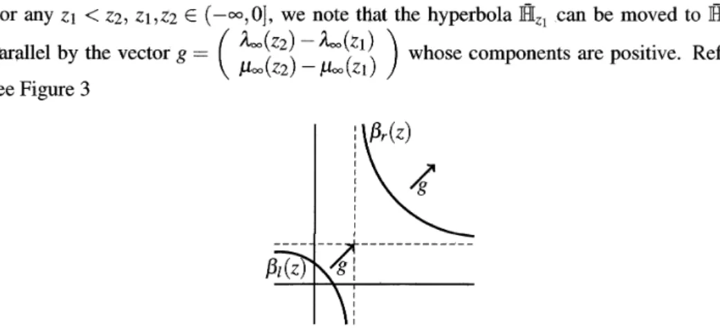
(6) 151 151. n-. \frac{a(0)}{b(0)}. z=0\Rightarrow z<0. Hyperbola I\overline{\mathb {H} _{0}. \frac{a(z)}{b(z)}. Hyperbola. \overline{\mathb {H}_{z}. Figure 2: Hyperbola \overline{\mathb {H} _{z}. Instead of the equation \delta_{r}(\lambda,\mu;z)=0 , relation (2.16) allows us to study the family of rect‐ angular hyperbola \mathb {H}_{z} indexed by z,i.e. equilateral hyperbola \mathb {H}_{z} on (\lambda,\mu) ‐plane, which is defined by. \mathbb{H}_{z}=\{(\lambda,\mu)\in \mathbb{R}^{2}|\mathbb{H}_{z}(\lambda,\mu)= 0\}. with asymptote (\lambda_{\infty}(z),\mu_{\infty}(z))=(a\{z)/b(z),n-z) . \mathbb{H}_{z}(\lambda,\mu) can be extended to z\in\langle-\infty\tau 0 ]. for any dimension n\geq 1 as. \overline{\mathb {H} _{z}(\lambda,\mu)=\{ begin{ar ay}{l } \mathb {H}_{z}(\lambda,\mu) , z<0, (\lambda-X)(\mu-n)-n, z=0. \end{ar ay}. (2.18). for n=1,2 and X=a(0)/b(0) for n\geq 3 . Refer to see Figure 2. Note that \overline{\mathbb{H} _{z}(0,0)=\frac{1}{b(z)}>0 for z<0 . We also extend the family of hyperbola \mathbb{H}_{z}, z\in(-\infty,0) , to. Here. X=1. that of hypertJola \overline{\mathb {H}_{z} indexéd by z\in(-\infty,0] by. \overline{\mathbb{H} _{z}=\{(\lambda,\mu)\in \mathbb{R}\cross \mathbb{R} |\overline{\mathbb{H} _{z}(\lambda,\mu)=0\}. For any. Z1<Z2,. Z1,Z2\in(-\infty,0], we note that the hyperbola \overline{\mathb {H} _{z_{1} can be moved to \overline{\mathb {H} _{z_{2} in. parallel by the vector see Figure 3. g=(\begin{ar ay}{l \lambda_{\infty}(Z2)-\lambda_{\infty}(z_{1}) \mu_{\infty}(Z2)-\mu_{\infty}(Z1) \end{ar ay}). Figure 3: Hyperbola \overline{\mathb {H} _{z} moves as. whose components are positive. Refer to. z. approaches to. -\infty. from. 0..
(7) 152 Let \beta_{l}(z) (resp. \beta_{r}(z) ) denote the left brunch (resp. the right brunch) of the hyperbola \overline{\mathb {H}_{z} , i.e. \overline{\mathbb{H} _{z}=\beta_{l}(z)\cup\sqrt{}t(z) , where U denotes the disjoint union. We then see that for any Z2<Z1\leq 0 it follows that \beta_{l}(z1)\cap\beta_{l}(z2)=\emptyset and \beta_{r}(z1)\cap\beta_{r}(z2)=\emptyset.. Lemma 2.4 Itfollows that. =\{ \infty 1-\mu (\lambda,\mu)\in mathb{H}_{0(\lambda,\mu)\not\inoverline{\mathb{H}_{0-} (n=2) \lim_{zarrow 0-}\delta_{r}(\lambda,\mu;z) =\{ \infty 1-\mu/2 (\lambda,\mu)\in mathb{H}_{0(\lambda,\mu)\not\in overline{\mathb{H}_{0-} (n \geq 3) \lim_{zarrow 0-}\delta_{r}(\lambda,\mu;z) =b(0) \overline{\mathb {H} _{0}(\lambda,\mu) . (n=1) 1_{\dot{4} m_{zarrow 0-}\delta_{r}(\lambda,\mu;z). Proof: In the case of n\geq 3 it is trivial to see that we consider cases of n=\varepsilon 1,2 . We recall that. \lim_{zarrow 0-}\delta_{r}(\lambda,\mu;z)=b(0)\overline{\mathbb{H} _{0} (\lambda,\mu) .. \delta_{r}(\lambda,\mu;z)=\gamma(z)\overline{\mathbb{H} _{z}(\lambda,\mu)= \gamma(z)\overline{\mathbb{H} _{0}(\lambda,\mu)+\gamma(z)(\overline{\mathbb{H} _ {z}(\lambda,\mu)-\ovalbox{\t \small REJECT}_{0}(\lambda,\mu)) and. \gamma(z)=b(z)=a(z)-\frac{1}{n}-\frac{1}{n}za(z). .. We can also directly see that for n=1,2. \overline{\mathb {H} _{z}(\lambda,\mu)\ovalbox{\t \smal REJECT} \overline{\mathb {H} _{0}(\lambda,\mu)=-\frac{1}{nb(z)}(1+za(z) (\mu-n)+ z(\lambda-\frac{a(z)}{b(z)}. .. Together with them we have. \delta_{r}(\lambda,\mu;z)=(a(z)-\frac{1+za(z)}{n})\overline{\mathbb{H} _{0} (\lambda,\mu)+\frac{a(z)}{b(z)}(1+za(z) (\frac{n-\mu}{n})+\xi, where. \xi=-Za(z)(\lambda-\frac{a(z)}{b(z)})+\frac{1+za(z)}{n}(\frac{(1+za(z) (\mu-n) }{nb(z)}+z(\lambda-\frac{a(z)}{b(z)}) It is well lmown in [5J that. a(z)= \frac{1}{\sqrt{-z}\sqrt{2-z} , n=1, a(z)=- \frac{\sqrt{2} {2\pi}\ln(-z)+(\frac{1}{2}-\frac{\sqrt{2} {\pi})+O(-z). ,. as. zarrow 0-,. By this it is crucial to see that. z ar ow 0-\frac{a(z)}{b(z)}=1. z arrow 0-hmza(z)=D, zarrow 0-1\dot{m}b(z)=\infty, \lim and. z ar ow 0-hm\xi=0, \lim_{zar ow 0-}\frac{a(z)}{b(z)}(1+za(z) (\frac{n-\mu}{n})- ar ow 1-\frac{\mu}{n}. n=2.. .. Then.
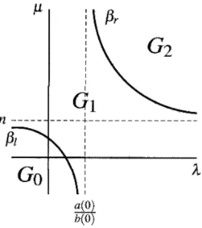
(8) 153 for n=1,2 . Let n=1 . Then. \delta_{r}(\lambda,\mu;z)=(a(z)-1-za(z) \overline{\mathbb{H} _{0}(\lambda,\mu) +\frac{a(z)}{b(z)}(1+za(z) (1-\mu)+\xi and the corollary follows fot n=1 . Let. n=2 .. In a similar manner to the case of. n=1. we. have. \delta_{r}(\lambda,\mu;z)=(a(z)-\frac{1+za(z)}{2})\overline{\mathbb{H} _{0} (\lambda,\mu)+\frac{a(z)}{b(z)}(1+za(z) (1-\frac{\mu}{2})+\xi, and the corollary foılows for n=2 . Hence the proof of the corollary can be derived. We define \overline{\delta}_{r}(\lambda,\mu;z\rangle for z\in(-\infty,0] by. \overline{\delta}_{r}(\lambda,\mu;z)=\{\begin{ar ay}{l } \delta_{r}(\lambda,\mu;z) , z\in(-\infty,0) , \lim_{zar ow 0-}\delta_{r}(\lambda,\mu;z), z=0. \end{ar ay} From Lemma 2.4 we can see that. (2.19). \overline{\delta}_{r}(\lambda,\mu;z) converges to. \overlin{\delta}_{r(\lambda,\mu;0)=\{begin{ar y}{l 1-\mu, n=1,(\lambda,\mu)\inoverlin{\mathb{H}_{0, 1-\mu/2, n=2,(\lambda,\mu)\inoverlin{\mathb{H}_{0, n\geq3,(\lambda,\mu)\inoverlin{\mathb{H}_{0. \end{ar y} Then we can show the continuity of. \overline{\delta}_{r}(\lambda,\mu;z). (2.20). on z :. Lemma 2.5 Itfollows that. (n=1,2)\overline{\delta}_{r}(\lambda,\mu;z) is continuous in z\in(-\infty,0] for (\lambda,\mu)\in\overline{\mathbb{H} _{0}, (n\geq 3)\overline{\delta}_{r}(\lambda,\mu;z) is continuous in z\in(-\infty,0 ] for (\lambda,\mu)\in \mathbb{R}^{2}. We set \beta_{l}=\beta_{l}(0) and \sqrt{}r=\beta_{r}(0) . The bmnches \beta_{I} and \beta_{r} of the hyperbola \overline{\mathb {H}_{0} split \mathb {R}^{2} into three open sets. G_{0}=\{(\lambda,\mu)\in \mathbb{R}^{2^{-} |\mathbb{H}_{0}(\lambda,\mu)>0, \lambda<\lambda_{\infty}(0)\}, G_{1}=\{(\lambda,\mu)\in \mathbb{R}^{2}|\mathbb{H}_{0}(\lambda,\mu)<0\}-, G_{2}=\{(\lambda,\mu)\in \mathbb{R}^{2}1\mathbb{H}_{0}(\lambda,\mu)>0, \lambda>\lambda_{\infty}(0)\}-. Refer to see Figure 4. Hence \partial G_{0}=\beta_{\iota} and \partial G_{2}=\beta_{r} follow.. \overline{\delta}_{r}(\lambda,\mu;z)\neq 0 for z\in(-\infty,0) . \overline{\delta}_{r}(\lambda,\mu;0)\neq 0forn=1,2. 3. Let (\lambda,\mu)\in\beta_{l} . Then \overline{\delta}_{r}(\lambda,\mu;0)=0 for n\geq 3.. Lemma 2.6. 2. Let. (2). (1). 1. Let (\lambda,\mu)\in G_{0}\cup\beta_{l} . Then. (\lambda,\mu)\in\beta_{l} . Then. 1. Let (\lambda,\mu)EG_{1}\cup\beta_{r} . Then \exists_{1}z\in(-\infty,0) such that. 2. Let (\lambda,\mu)E\beta_{r} . Then 3. Let. (\lambda,\mu)\in\beta_{r} . Then. \overline{\delta}_{r}(\lambda,\mu;z)=0.. \overline{\delta}_{r}(\lambda,\mu;0)\neq 0 for n=1,2. \overline{\delta}_{r}(\lambda,\mu;0)=0forn\geq 3.. (3) Let (\lambda,\mu)\in G_{2} . Then \exists z1,Z2\in(\propto\infty,0) such that. \overline{\delta}_{r}(\lambda,\mu;z1)=\overline{\delta}_{r}(\lambda,\mu;_{Z2})= 0..
(9) 154 Proof: Let (\lambda,\mu)\in G_{0}U\beta_{l} . Then we can see that (\lambda,\mu)\not\in\overline{\mathbb{H} _{z} for any z\in(-\infty,0) . Thus (1)1 follows. Also it can be seen that U_{z\in(-\infty,0)}\beta_{J}(z)\supset G_{1} , \beta_{l}(z)\cap\beta_{l}(w)=\emptyset if z\neq w , and. \beta_{r}(z)\cap G_{1}=\emptyset. Hence there exists a unique z\in\langle-\infty,0) such that (\lambda,\mu)\in\beta_{l}(z) , which. proves (2)1. We can also see that U_{z\in(-\infty,0)}\beta_{l}(z)\supset G_{2}, \bigcup_{z\in(-\infty,0)}\beta_{r}(z)\supset G_{2}, \beta_{l}(z)\cap\beta_{l}(w)= \emptyset if z\neq w, \beta_{r}(z)\cap\beta_{r}(w)=eifz\neq w , and \sqrt{}l(z)\cap\beta_{r}(z)=\emptyset . Hence there exist Z1,Z2\in(-\infty,0). such that (\lambda,\mu)\in\beta_{l}(z1) and (\lambda,\mu)\in\beta_{r}(z2) , which proves (3). Finally we note that since (\lambda,\mu)\in\beta_{I} implies that 1\neq\mu for n=1 , and 2\neq\mu for n=2,\overline{\delta}_{r}(\lambda,\mu;0)\neq 0 for n=1,2 follows. Hence (1) 2 and (1) 3 follow from (2.20), and (2) 2 and (2) 3 are similarly proven. qed. \perp a0) b(0). Figure 4: Region of G_{j} By virtue of Lemma 2.6,. \overline{\delta}_{r}(\lambda,\mu;\cdot) has at most two zeros in (-\infty,0) .. Lemma 2.7 Let n\geq 1 . Then (1) and(2) follow.. (1) Let \lambda\neq 0 . We assume that z_{1,Z2}\in(-\infty,0) and \delta_{r}(\lambda,\mu;_{Zk})=0 (if they exist). Then , 1-\mu a(zk)\neq 0 and G_{+}(z_{k})Z_{k}=Z_{k} has the solutions: k=1,2, and the corresponding eigenfunctions,. Z_{k}=( \frac{\lambda}{\sqrt{2} \frac{nb(z_{k})}{1-\mu a(z_{k})}, 1, \cdots, 1). H_{\lambda\mu}^{+}f_{k}=zf_{k}, are. f_{k}(p)=- \frac{1}{(2\pi)^{n/2} \frac{i}{E(p)}\overline{\sqrt{2}∽\lamZbkd(a\mu\frac{nb(z_{k}) {1-\mu a(z_{k}) +\sum_{]=1}^{n}\cos p_{j}) ,. k=1,2 .. (2.21). (2) Let \lambda=0 . We assume that z\in(-\infty,0) and \delta_{t}(0,\mu;z)=0 . Then 1-\mu a(z)=0 and G_{+}(z)Z=Z has the solution: Z=(1, \sqrt{2}\mu b(z), \cdots, \sqrt{2}\mu b(z))^{T} and the corresponding. eigenfunction,. H_{\lambda\mu}^{+}f=zf, is. f(p)= \frac{\mu}{(2\pi)^{n/2} \frac{1}{E(p)-z} Proof: We prove the case of n\geq 2 . The proof for the case of. \delta_{r}(\lambda,\mu;z)=0 , we see that. (2.22) n=1. is similar. Since. (1-\mu a(z))(1-\lambda(c(z)+(n-1)d(z)))-n\lambda\mu b^{2}(z)=0..
(10) 155 Then 1-\mu a(z)\neq 0 if and only if \lambda\neq 0 , and we also have the algebraic relation. 1- \lambda(c(z)+(n-1)d(z) =\frac{n\lambda\mu b^{2}(z)}{1-\mu a(z)}. From this relation it follows that G_{+}(zk)Z_{k}=Z_{k} for \lambda\neq 0 . In the case of \lambda=0 we can prove the lemma in a similar way. qed. We study zeros of \delta_{c}(\lambda;z) . In a similar manner we extend \delta_{c}(\lambda,z) for z\in(-\infty,0 ].. Wllen n\geq 2 , the function c(z)-d(z) exists, and we can define \alpha=\lim_{zarrow 0-}c(z)-d(z) . Note that \alpha>0 and we set \lambda_{c}=\frac{1}{\alpha} . Let us write \delta_{c}(\lambda;z)=p(\lambda;z)^{n-1} , where p(\lambda;z)=. \lambda(c(z)-d(z))-1 . We define \overline{\delta}_{c}(\lambda;z) by. \overline{\delta}_{c}(\lambda;z)=\{ begin{ar y}{l \delta_{c}(\lambda;z), z\in(-\infty,0)n\geq1, (\lambda\ lpha-1)^{n-1}, Z=0,n\geq2, 1, z=0,n=1. \end{ar y} Lemma 2.8 Let n\geq 2. Then (1) -(3) follow. (1) Let \lambda<\lambda_{c} . Then p(\lambda;z)\neq 0 for any. \lambda^{-}>\lambda_{c} . Then there exists unique. z\in(-\infty,0) . (2) Let \lambda=\lambda_{c} . Then \rho(\lambda;0)=0. (3) Let z\in(-\infty,0) such that p(\lambda;z)=0 with multiplicity one.. Proof:. Since. c(Z)-d(z)>0 is strictly monotone increasing in (-\infty,0) , we get. p(\lambda;z)\leq p(\lambda_{\kappa};z)<\rho(\lambda_{c};0)=0 ,. p(\lambda;z)=-1 ,. if. 0<\lambda\leq\lambda_{c},. if. \lambda\underline{\neg}0,. which prove (1) and (2). Since \rho(\lambda;0)>\rho(\lambda_{c};0)=0 and hm_{zarrow-\infty}\rho(\lambda;z)\overline{arrow}-1 there exists z\in(-\infty,0) sUch that \rho(\lambda;z)=0 . By the monotonicity of p(\lambda;\cdot) this zero ís a unique and has multiplicity one. Hence (3) is proven. qed We immediately have a lemma. Lemma 2.9 Let n\geq 2. Then (1) -(3) follow. (1) For any. \lambda\leq\lambda_{c},\overline{\delta}_{c}(\lambda;\cdot) has no zero in (-\infty,0) .. (2) Let \lambda=\lambda_{c} . Then. \overline{\delta}_{c}(\lambda;0)=0, and. z=0. has multiplicity. n-1.. (3) For any \lambda>\lambda_{c},\overline{\delta}_{c}(\lambda;\cdot) has a unique zero in (-\infty,0) with multiplicity. n-1.. Next we show the eigenfunction corresponding to zeros of \delta_{\mathcal{C} (\lambda;\cdot) , Lemma 2.10 Let n\geq 2, z\in(-\infty,0) and. of G_{+}(z)Z=Z are given by corresponding eigenfiunctions,. \overline{\delta}_{c}(\lambda;z)=0 .. I.e.,. Z_{j}=(0,1,0, \cdots,-1,\cdot,0)^{T}j+2..,. \lambda=\frac{1}{c(z)-d(z)} .. H_{\lambda\mu}^{+}g_{j}=zg_{j}, are. g_{j}(p)= \frac{\lambda}{\sqrt{2} \frac{1}{(2\pi)^{n/2} \frac{1}{E(p)-z}(\cos p_{1}-\cos p_{j+1}) ln partícular the multiplicity of eigenvalue. z. is at least. ,. n-1.. j=1,. j=1 , ...,. Then the solutions. n-1 ,. n-1 .. and hence the. (2.23).
(11) 156 Now we study the spectrum located on the left edge of the essential spectrum [0,2n] , i.e., Suppose that (\lambda,\mu)\in\overline{\mathbb{H} _{0} . Then it is possibıy \overline{\delta}_{r}(\lambda,\mu;0)=0 or \overline{\delta}_{c}(\lambda,\mu;0)=0 . We. z=0_{\backslash }. study zeros of for n\geq 3.. \overline{\delta}_{r}(\lambda,\mu;0) for. n\geq 3 . We set. Lemma 2.11 Let n\geq 3 . (1) Let \lambda\neq 0 and. has the solution. Z=. solution:. a(0)=a and b(0)=b, and both a and b are finite. \overline{\delta}_{r}(\lambda,\mu;0)=0 .. Then 1-\mu a\neq 0 and G_{+}(0)Z=Z. ( \frac{\lambda}{\sqrt{2} \frac{nb}{1-\mu a}, 1, \cdots , 1)^{T} and the corresponding equation H_{\lambda\mu}^{+}f=0 has the. f(p)= \frac{\lambda}{\sqrt{2} \frac{1}{(2\pi)^{n}f^{2} \frac{1}{E(p)} (\mu\frac{nb}{1-\mu a}+\sum_{j=1}^{n}\cos p_{j}). .. (2.24). (2) Let \lambda=0 and \delta_{r}(0,\mu;0)=0 . Then 1-\mu a=0 and G_{+}(0)Z=Z has the solufion:. Z=(1,0, \cdots,0)^{T} and the corresponding equation H_{\lambda\mu}^{+}f=0 has the solution:. f(p)= \frac{\mu}{(2\pi)^{n/2} \frac{1}{E(p)}. .. (2.25). Proof: The proof is the same as that of Lemma 2.7. Next we show the solution. c(). qed. rresponding to zeros of 5_{c}(\lambda;\cdot) . Similar to the case of. \delta_{r}(\lambda,\mu;z)=0 , we have the lemma below.. Lemma 2.12 Let n\geq 2 and \delta_{c}(\lambda;0)=0, i.e.) \lambda=\lambda_{c} . Then the solutions of G_{+}(0)Z=Z j+2. are given by Z_{j}=(0,1,0, \cdots, -1, \cdots,0)^{T}, j=1, equation. H_{\lambda\mu}^{+}g_{j}=0. n-1 ,. and hence the corresponding. has the solutions. g_{j}(p)= \frac{\lambda_{c} {\sqrt{2} \frac{1}{(2\pi)^{n/2} \frac{1}{E(p)}(\cos p_{1}-\cos p_{j+1}) Proof: The proof is the same as that of Lemma 2.10.. ,. j=1 , ...,. n-1 .. (2.26). qed. As was seen above the problem for n\geq 3 can be reduced to study the spectrum of G+ by the Birman‐Schwinger principle, the problem fdrn=1,2 should be however directly investigated.. As was seen above the problem for. n\geq 3. can be reduced to study the spectrum of G_{e}. by the Birman‐Schwinger principle, the problem for n=I,2 should be however directly investigated. Let f be a solution of. H_{\lambda\mu}^{+}f=0 (resp. H_{\lambda}^{-}f=0) (1) If f\in L_{+}^{2} (resp. f\in L^{\underline{2} ), we say that is a threshold eigenvalue of H_{\lambda\mu}^{+} (resp. H_{\lambda}^{-} ). (2) If f\in L_{+}^{1}\backslash L_{+}^{2} (resp. f\in L^{\underline{1} \backslash L^{\underline{2} ), we say that 0 is a threshold resonance of H_{\lambda\mu}^{+} (resp. H_{\lambda}^{-} ). (3) If f\in L_{+}^{\varepsilon}\backslash L_{+}^{1} (resp. f\in L^{\underline{\varepsilon} \backslash L^{\underline{1} ) for any O1 , we say that 0 is a super‐threshold resonance ofH_{\lambda\mu}^{+} (resp. H_{\overline{\lambda} ). 0. Lemma 2.13 Let n=1.. (1) Suppose that f\in L^{1}(\mathbb{T}) and H_{\lambda\mu}^{e}f=0 . Then f=0. In panicularH_{\lambda\mu}^{e} has no threshold resonance..
(12) 157 (2) There is no non‐zero f such that f\in L^{\varepsilon}(\Gamma^{2})\backslash L^{1}(\Gamma^{2}) for some In particular H_{\lambda\mu}^{e} has no super‐threshold resonance.. Proof: (1). 0<\varepsilon<1andH_{\lambda\mu}^{e}f=0.. H_{\lambda\mu}^{e}f=0 gives f=\varphi/E and \varphi(p)=\mu u_{0}+\lambda u_{1}\cos p by (2.2).. it follows that. From f\in L^{1}(\Gamma). \varphi(0)=\mu u_{0}+\lambda u_{1}=0 . Hence. f(p)= \frac{1}{E(p)}(1-\cos p)\mu u_{0}=\mu u_{0}. We get (2). u1= \mu u0\frac{{\imath}}{2\pi}\int_{\Gamma}\cos tdt=0 , which gives. S i nce. \mu u0=0 and f=0. f\not\in L^{1}(\Gamma) . It must be that \mu=0 and f=\varphi/E with \varphi(p)=\lambda u_{1}\cos p . Hence. u_{1}= \frac{\lambda}{(2\pi)^{2} \int_{\Gamma}\frac{u_{1}o s^{2}p}{E(p)}dp. Then u_{1}=0 , since. \int_{\Gamma}\frac{\cos^{2}p}{E(p)}dp=\infty . Then. f=0 follows.. Next we discuss the spectrum of H_{\lambda\mu}^{e} for. n=2. at the threshold. Lemma 2.14 Let n=2.. (1) Suppose that. f\in L^{1}(\mathbb{T}^{2}) and H_{\lambda\mu}^{e}f=0 .. Then \lambda=\lambda_{c} and. f(p)= \lambda_{c}u_{1}\frac{cosp_{1}-cosp_{2} {E(p)} . ln particular. (2.27). f\in L^{2}(\Gamma^{2}) and H_{\lambda\mu}^{e} has no threshold resonance.. (2) There is no non‐zero f such that f\in L^{\varepsilon}(\Gamma^{2})\backslash L^{1}(\mathbb{T}^{2}) for some In particular H_{\lambda\mu}^{e} has no super‐threshold resonance.. 0<\varepsilon<1andH_{\lambda\mu}^{e}f=0.. L^{1}(T^{2}) . We can take f=\varphi/E and \varphi(p)=\mu u_{0}+ \lambda u_{1}\cos p_{1}+\lambda u_{2}\cos p_{2} . Since f\in L^{1}(\mathbb{T}^{2}), we get \varphi(0)=\mu u_{0}+\lambda(u_{1}+u_{2})=0 and so. Proof‘. (1) Consider. H_{\lambda\mu}^{e}f=0. in. f(p)= \frac{\lambda}{E(p)}(-u_{1} (1 ‐cos p_{1})-u_{2}(1-\cos p_{2})) We obtain. u_{1}=- \frac{\lambda}{(2\pi)^{2} (u_{1}\int_{\mathb {P} \frac{\cos p_{1}(1- \cos p_{ \imath} )}{E(p)}dp+u2\int_{\Gamma^{2} \frac{\cos p_{1}(1-cosp_{2})} {E(p)}dp) u_{2}=- \frac{\lambda}{(2\pi)^{2} (u_{ \imath} \int_{\Gamma^{2} \frac{cosp_{2} (1-\cos p_{1})}{E(p)}dp+u_{2}\int_{\Gamma^{2} \frac{\cos p_{2}(1-\cos p_{2})} {E(p)}dp) S i nce. \int_{\Gamma^{2} \frac{\cos p_{1}(1-\cos p_{1})}{E(p)}dp=-\int_{\Gamma^{2} \frac{\cos p_{1}(1-\cos p_{2})}{E(p)}dp, we get. u_{1}= \frac{\lambda}{(2\pi)^{2} (u_{2}-u_{1})(\int_{\Gamma^{2} \frac{\cos p_{1}(1-\cos p_{1})}{E(p)}dp) u_{2}= \frac{\lambda}{(2\pi)^{2} (u_{1}-u_{2})(\int_{\Gamma^{2} \frac{\cos p_{2}(1-\cos p_{2})}{E(p)}dp). ,. ,. ..
(13) 158 and hence. u_{1}=-u_{2} .. Consequently, \mu u_{0}=0 , and the solution of H_{\lambda\mu}^{e}f=0 is of the form. f(p)= \lambda u_{1}\frac{\cos p_{1}-\cos p_{2} {E(p)}\in L^{2}(\Gamma^{2}) . Inserting this into the definition of. u_{I} ,. we have. (2.28). \frac{a}{(2\pi)^{2} \int_{\Gamma^{2} \frac{\cos p_{1}(\cos p_{1}-\cos p_{2})} {E(p)}dp=1 and thus. taking \lambda=\lambda_{c} we can see that (2.27) is the solution of H_{\lambda\mu}^{e}f=0 . Notice that u_{0}=0 follows from (2.28). (2) Since f\not\in L^{1}(\Gamma^{2}) . It must be that \mu=0 and f=\varphi/E with \varphi(p)=\lambda u_{1}\cos p_{1}+. \lambda u_{2}\cos p_{2} .. Hence. u_{1}= \frac{\lambda}{(2\pi)^{2} \int_{\mathb {T}^{2} \frac{u_{1}\cos^{2}p_{1}+ u_{2}\cos p_{1}\cos p_{2} {E(p)}dp, u_{2}=- \frac{\lambda}{(2tr)^{2} \int_{\mathb {T}^{2} \frac{a1^{\cos p2^{\cos} Pt^{+u_{2}\cos^{2_{P2} } {E(p)}dp. Then. u_{1}=-u_{2}. (2.28), but. and. 1= \frac{\lambda}{(2\pi)^{2} \int_{\Gamma^{2} \frac{\cos p_{1}(\cos p_{1}+\cos p_{2})}{E(p)}dp .. Thus \lambda=\lambda_{c} . Then f is given by. f\in L^{2}(\Gamma^{2}) . This contradicts with f\not\in L^{1}(\Gamma^{2}) .. Lemma 2.15 (1)‐(5) follow: (1) Let. n=1 .. Then. 0. is none of a threshold eigenvalue, a threshold. resona\eta ce. and a. super‐threshold resonance.. (2) Let. n=2.. Thpn. 0. multiplicity is one.. is a threshold eigenvalue with (2.26) for (\lambda,\mu)=(\lambda_{c},\mu) and its. (3) Let n=3,4 , Suppose (\lambda,\mu)\in \mathbb{H}_{0} . Then 0 is a threshold resonance with eigenvector (2.24) for \lambda\neq 0, and (2.25) for \lambda=0, i. e., (\lambda,\mu)=(0,1/a) .. (4) Let n=3,4 . Suppose (\lambda,\mu)\in \mathbb{H}_{0} . Then \lambda=\lambda_{c} and its with multiplicity is n-1.. 0. is a threshold eigenvalue with (2.26) for. (5) Let n\geq 5 . Suppose (\lambda,\mu)\in \mathbb{H}_{0} . Then 0 is a threshold eigenvalue with eigenvector (2.24)for \lambda_{c}\neq\lambda\neq 0 and multiplicity one, (2.24) and (2.26)for \lambda=\lambda_{c} and multiplicity n , and (2.25) for \lambda=0, i. e., (\lambda,\mu)=(0,1/a) , and multiplicity one.. Proof: (1) follows from Lemma2.13. The solution of H_{\lambda\mu}^{+}f=0 is given by (2.24), (2.25) and (2.26). We note that \int_{|p|<\varepsilon}\frac{1}{E^{2}(p)}dp=\infty for n=2,3,4 for any \varepsilon>0 , and \int_{|p|<\varepsilon}\frac{1}{E^{2}(p)}dp<\infty for n\geq 5 for any. \varepsilon>0. S i n ce. (\lambda,\mu)\in\overline{\mathbb{H} _{0}, n\neq\mu , and we can see that. \frac{nb\mu}{1-\mu a}+\sum_{j=1}^{n}\cos 0=\frac{nb\mu}{1-\mu a}+n\Rightar ow n(\frac{1-\mu(a-b)}{1-\mu a})=\frac{n-\mu}{1-\mu a}\neq 0. Hence, using Lemma 2.2, we obtain (2.24), (2.25)\in L^{2} for n\geq 5, (2.24),(2.25)\in L^{1}\backslash L^{2} for n=3,4 and (2.26)\in L^{2} for n\geq 2 . (2) follows from Lemmas 2.14 and 2.12. (3) and (5) follow from Lemmas 2.12 and 2.11. (4) follows from Lemma 2.12. qed.
(14) 159 3. Spectrum of odd part H_{\lambda}^{-}. In the previous sections, we study the spectrum of H_{A\mu}^{+} by using the Binnan‐Schwinger principle for n\geq 3 , and by directly solving H_{\lambda\mu}^{+}f=0 for n=1,2 . In the case of H_{\lambda}^{-} we can proceed in a similar way to the the case of H_{\lambda\mu}^{+} and rather easier than that of H_{\lambda\mu}^{+} as is seen. below. Let z\in \mathbb{C}\backslash [0,2n] . Let N_{n} be the linear hull of. \{s_{1} ,s_{n}\} .. As is done for. can see that (H_{0}-z)^{-1}V_{\lambda}^{-}=S_{1}S_{2} . Here S_{1} and S_{2} are defined by S_{1}. :. H_{\lambda\mu}^{+} , we. \mathb {C}^{n}\ni(w_{1}, \cdots fw_{n})\mapsto(H_{0}-z)^{-1}\frac{\lambda}{2} \sum_{j=1}^{n}w_{j}s_{j}\in L_{-}^{2},. S_{2}:L^{\underline{2} \ni\psi\mapsto(\langle\phi,s_{1}\rangle, \cdots, \{\phi, s_{n}\rangle)\in \mathbb{C}^{n}. We set G_{-}(z)=S_{2}S_{1} :. \mathbb{C}^{n}arrow \mathbb{C}^{n} .. The following assertion is proved as Lemma 2.1.. Lemma 3\cdot 1 (Birman‐Schwinger principle for z\in \mathbb{C}\backslash [0,2n] ). (1) z\in \mathbb{C}\backslash [0,2n] is an eigenvalue of H_{\overline{\lambda} if and only if 1\in\sigma(G_{-}(z)) . (2) Let z\in \mathbb{C}\backslash [0,2n1andZ=(w_{1}, \ldots,w_{n})^{T}\in \mathbb{C} ^{n} be such that G_{-}(z)Z=Z. Then f=s_{1}z,. f(p)= \frac{1}{(2\pi)^{n/2} \frac{1}{E(p)-z}(\frac{\lambda}{\sqrt{2} \sum_{j=1} ^{n}w_{j}\sin p_{j}) is an eigenfunction of H_{\lambda}^{-} , i. e., H_{\lambda}^{-}f=zf.. We see that G_{-}(z)=\lambda s(z)I . Consequently we have for n\geq 1, \delta_{s}(\lambda;z)=\det(G_{-}(z)-I)= (\lambda s(z)-1)^{n} . Since G_{-}(Z) is diagonal, it is very easy to find solution of G_{-}(z)Z=Z . It has n independent solutions: Z_{j}=(0. is given by. ,. 1,\cdot 0\rangle^{T}\dot{f}. .. The corresponding eigenvector, H_{\overline{\lambda}}f_{j}=zf_{j},. f_{j}(p)= \frac{1}{E(p)-z}\frac{1}{(2\pi)^{n/2} \frac{\lambda}{\sqrt{2} \sin p_ {j},. j=1,. \ldots,n ,. (3.1). where \lambda=1/s(z) . In particular the multiplicity of z is n . We can extend the Bihman‐ Schwinger principle for z=0 . We extend the eigenvalue equation H_{\lambda}^{-}f=0 in L^{\underline{2} to that in. L^{\underline{1} . Wé consider the equation. E(p)f(p)- \frac{\lambda}{(2\pi)^{n} \sum_{j=r}^{n}s np_{j}\int_{\Gamma^{n} \sin p_{j}f(p)dp=0 i. (3.2). in L^{\underline{1} . We also describe (3.2) as. H_{\lambda}^{-}f=0 . We can see that s i np_{j}/E(p)\approx 1/|p| in the neighborhood of p=0 , and then s i np_{j}fE(p)\in L^{1} for n\geq 2 . By (5) of Lemma 2.2 and V_{\lambda}^{-}f\in C we can see that. L^{\underline{2} \ni f\mapsto H_{0}^{-1}V_{\lambda}^{+}f\in L_{-}^{2}, L^{\underline{1} \ni fi\mapsto H_{0}^{-1}V_{\lambda}^{-}f\in L_{-}^{1},. n\geq 3 ,. (3.3). n\geq 2 .. (3.4).
(15) 160 Thus for n\geq 2 we can extend operators S_{1} and S_{2} . Let n\geq 2 and Z \mathbb{C}^{n}ar ow L^{\underline{1} is defined by. =. ( wı,. ,. w_{n})^{T}.\overline{S}_{1} :. \overline{S}_{1}Z=\frac{1}{(2\pi)^{n/2} \frac{\lambda}{\sqrt{2} \frac{1}{E(p)} \sum_{j=1}^{n}w_{j}\sin p_{j} and \overline{S}_{2} : L^{\underline{1} ar ow \mathbb{C}^{n} by. \overline{S}_{2}:L^{\underline{1} \ni\psi\mapsto(\int_{T^{n} \phi(p)s_{1}(p) dp, \ldots, \int_{T^{n} \phi(p)s_{n}(p)dp)^{T}\in \mathbb{C}^{n}. Then \overline{S}_{1}\overline{S}_{2} : L^{\underline{1} ar ow L^{\underline{1} . Consequently. G_{-}(0)=\overline{S}_{2}\overline{S}_{1} : \mathbb{C}^{n}arrow \mathbb{C}^{n} is described as an n\cross n matnix.. Let n\geq 2 . We have (1) \lim_{zarrow 0}G_{-}(z)=G_{-}(0) , and (2) Hence for. n. 〉 2,. \sigma(H_{0}^{-1}V_{\lambda}^{-})\backslash \{0\}=\sigma(G_{-}(0) \backslash \{0\}.. G_{-}(0)=\lambda s(0)I and. (3.5). \overline{\delta}_{s}(\lambda;z) is defined by. \overline{\delta}_{s}(\lambda;z)=\{\begin{ar ay}{l } \delta_{s}(\lambda;z) z\in(-\infty,0) , (\lambda s(0)-1)^{n} z=0. \end{ar ay}. (3.6). Lemma 3.2 (Birman.Schwinger principle for z=0 ) Let n\geq 2 . Then (1) and (2) follow. (1) Equation H_{\lambda}^{-}f=0 has a solution in L^{i} if and only if 1\in\sigma(G_{-}(0)) . (2) Let Z= (W_{1}, \ldots, w_{n})^{T}\in \mathbb{C}^{n} be the solution of G_{-}(0)Z=Z ifand only if f=\overline{S}_{1}Z, i. e.,. f(p)= \frac{1}{(2\pi)^{n} \frac{1}{E(p)}\frac{\lambda}{\sqrt{2} \sum_{j=1}^{n} w_{j}s is a solution of H_{\overline{\lambda}}f=0, where. i np_{j}. w_{j}= \frac{\sqrt{2} {(2\pi)^{n/2} \int_{\Gamma^{n} f(p)si np_{j}dp,. j=1,. n.. Proof. The proof is the same as that of Lemma 2.3.. qed. \cdot. Set. \lambda_{s}=\frac{1}{s(0)}.. Lemma 3.3 Let h\geq 1 . Then (1)‐(3) follow: (1) Let \lambda\leq\lambda_{s}. Then. \overline{\delta}_{s}(\lambda;\cdot) has no zero ín (-\infty,0) .. (2) Let \lambda=A_{s} . Then. \overline{\delta}_{s}(\lambda_{s};0)=0 and. (3) Let \lambda>\lambda_{s} . Then. \overline{\delta}_{s}(\lambda;\cdot) has a unique zero in (-\infty,0) with multiplicity. z=0 has multiplicity. n.. Proof: The proof is similar to that Qf Lemma 2.9, and hence we omit it.. n.. qed. Threshold resonances and threshold eigenvalues for H_{\overline{\lambda} can be discussed by the Birman‐ Schwinger principle for n\geq 2.. Lemma 3.4 Let n\geq 2 . Then the solutions of equation H_{\lambda}^{-}f=0 are given by. f_{j}(p)= \frac{1}{(2\pi)^{n/2} \frac{\lambda_{s} {\sqrt{2} \frac{s\dot{m}p_{j} }{E(p)}, j=1, \ldots,n. .. (3.7).
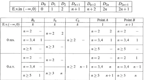
(16) 161 161 Proof: By For. \overline{\delta}(\lambda_{s},0)=0 and Lemma 3.2 the lemma follows.. n=1. qed. we can directly see that H_{\lambda}^{-}f=0 has no solution in L^{1} , but H_{\lambda}^{-} has a super‐. threshold resonance.. Proposition 3.5 (Super‐threshold resonance) Let. L^{\varepsilon}\backslash L^{1} for any. 0<\varepsilon<1 .. I.. e., 0. n=1 .. Then H_{\overline{\lambda}}f=0 has solution f\in is a super‐threshold resonance of H_{\lambda}^{-}.. Proof: H_{\lambda}^{-}f=0 yields that. f(p)= \frac{\lambda}{2\pi}\frac{s\dot{m}p}{E(p)}\int_{\Gamma}\sin pf(p)dp. Note that however s i np/E(p)\not\in L^{1} , but we can see that \sin p/E(p)\in L^{\varepsilon} for any since \sin p/E(p)\sim 1/p near p=0 and \int_{\Gamma}p^{-\varepsilon}dp<\infty .. Lemma 3.6. (1) Let. n=1 .. Then. 0. 0<\varepsilon<1. qed. is neither a threshold resonance and a threshold eigen‐. value, butfor (\lambda,\mu) with \lambda\neq 0,0 is a super‐threshold resonance. Then. 0. is a threshold resonance at \lambda=\lambda_{s}.. (3) Let n\geq 3 . Then. 0. is a threshold eigenvalue at \lambda=\lambda_{s} and its multiplicity is. (2) Let. n=2 .. n.. Proof‘ (1) follows from Proposition 3.5. Let n\geq 2 . Then the solution of H_{\lambda}^{-}f=0 is given by (3.7). Since for n=2 and for n\geq 3 , we have f\in L^{1}\backslash L^{2} for n=2 ,. 4 4.1. \frac{s\dot{m}p_{j} {E(p)}\in L^{1}\backslash L^{2}. and f\in L^{2} for. n\geq 3 .. \frac{s\dot{m}p_{j} {E(p)}\in L^{2}. Then (2) and (3) follow.. qed. Main theorems Case of. n\geq 2. In order to describe the main results we have to separate (\lambda,\mu) ‐plane into several regions.. Lemma 4.1 Let. n\geq 2 .. Then \lambda_{\infty}(z)\leq\lambda_{s}(z)\leq\lambda_{c}(z) for z\in(-\infty,0].. \lambda_{c}(z)=\frac{1}{c(z)-d(z)}>\lambda_{s}(z)=\frac{1}{s(Z)} >\lambda_{\infty}(z)=\frac{a(z)}{b(z)} for. Proof‘ It follows that argument the lemma follows.. z<0 .. By a limiting qed. Introduce four half planes:. \mathfrak{C}_{-}=\{(\lambda,\mu)\in \mathbb{R}^{2}|\lambda<\lambda_{c}\}\prime, \mathfrak{C}_{+}=\{(\lambda,\mu)\in \mathbb{R}^{2}|\lambda>\lambda_{c}\} \mathfrak{S}_{-}=\{(\lambda,\mu)\in \mathbb{R}^{2}|\lambda<\lambda_{s}\}, \mathfrak{S}_{+}=\{(\lambda,\mu)\in \mathbb{R}^{2}1\lambda>\lambda_{s}\}, and two vertical li n es: \mathfrak{S}_{-}\subset \mathfrak{C}_{-}. \beta_{c}=\{(\lambda,\mu)\in \mathbb{R}^{2}|\lambda=\lambda_{c}\} and \beta_{s}=\{(\lambda,\mu)\in \mathbb{R}^{2}|\lambda=\lambda_{s}\} .. Note that. and \mathfrak{C}_{+}\subset \mathfrak{S}+ , and we define open sets by. D_{0}\Rightarrow G_{0}, D_{1}=G_{1}\cap \mathfrak{S}_{-}, D_{2}=G_{2}\cap 6_{-} , D_{n+1}=G_{1}\cap(\mathfrak{S}+\cap \mathfrak{C}_{-}). D_{n+2}=G_{2}\cap(\mathfrak{S}_{+}\cap \mathfrak{C}_{-}) , D_{2n}=G_{1}\cap \mathfrak{C}+, D_{2n+1}=G_{2}\cap \mathfrak{C}+\cdot. ,.
(17) 162. Table 1: Spectrum of H_{\lambda\mu} for (\lambda,\mu) on D_{k} and the edges of D for n\geq 2. \mathb {H}_{0}. \lambda_{s} \lambda \lambda_{s} \lambda_{c}. n\geq 3 n=2. Figure 5: Hyperbola for. n. 〉‐ 2. The boundaries of these sets define disjoint eight curves:. B_{0}=\beta_{J}, B_{1}=\beta_{r}\Gamma t\mathfrak{S}_{-}, B_{n+1}=\beta_{r}\cap (\mathfrak{S}_{+}\cap \mathfrak{C}_{-}) , B_{2n}=\beta_{r}\cap \mathfrak{C}+, S_{1}=\beta_{s}\cap G_{1}, S_{2}=\beta_{s}\cap G_{2}, C_{n+1}=\beta_{c}\cap G_{1}, C_{n+2}=\beta_{c}\cap G_{2}, and two one point sets given by A=\beta_{r}\cap\beta_{s} and B=\beta_{r}\cap\beta_{c}. We are now in the position to state the main theorem for n\geq 2. Theorem 4.2 Let n\geq 2.. (1) Assume that (\lambda,\mu)\in D_{k}, k\in\{0,1,2,n+1,n+2,2n,2n+1\} , then H_{\lambda\mu} has k eigen‐ values in (-\infty,0) . Ifl addition H_{\lambda\mu} has neither a threshold eigenvalue nor a threshold resonance.. (2). 0. is not a super‐threshold resonance ofH_{\lambda\mu} for any. (\lambda,\mu)\in \mathbb{R}^{2}..
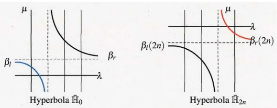
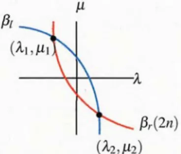
(18) 163 (3) Assume that (\lambda, \mu) in B_{k}, S_{k}, C_{k} and A,B resùlts in Table 4.1 are true:. Proof: (1) follows from Lemmas 2.6, 2.9 and 3.3. (2) follows from Lemmas 2.133.4 and 3.6. (3) follows from Lemmas 2.15 and 3.6. qed. As is drawn in Figures 5 and 9, hyperbolas for n=1,2 include the origjn \langle 0,0 ), which. is different from those for n\geq 3 . It actually describes that the Hamiltonian H_{\lambda\mu} with \lambda=0 has a negative eigenvaıue for any \mu>0 . This is clarified in e.g.,[3] and is also hold for one or two dimensional Schrödinger operator of the form -(1/2)\Delta+V ‐ We refer to see e.g., [6] and reference therein. Moreover for any (\lambda,\mu)\in(0,\infty)\cross(0,\infty), H_{\lambda\mu} always has negative eigenvalue and dose not have threshold resonance nor threshold eigenvalue fQrn=1,2. By a Rellich type theorem for the discrete Schödinger operator, embedded eigenvalues may be absent in the interval (0,2n) . Under some assumptions this is proven in [4]. We are however interested in constructing a Hamiltonian H_{\lambda\mu} which has two eigenvalues on both edges of the spectrum [0,2n] . See Figure 6 below:. Figure 6: Two embedded eigenvalues or resonances of H_{\lambda\mu}. By the discussion stated in the previous sections we can constmct an exampıe of discrete Schrödminger operators which has two embedded eigenvalues. Let n\geq 3 . Points (\lambda,\mu) on. the blue curve in the upper left construct Schrödinger operators H_{\lambda\mu} which has resonance or eigenvalue at 0 . On the other hand points (\lambda,\mu) on the red curve in the upper right construct. Schrödinger operators H_{\lambda\mu} which has resonance or eigenvalue at. \beta_{r}. Hyperbola \overline{H}_{0}. 2n .. See Figure 7.. 2n). \beta_{I}(2n. Hyperbola \overline{\mathb {H} _{2n}. Figure 7: Resonance and eigenvalue oh edges We have the theorem.. Tlleorem 4.3 (1) Let n=3,4 . Then there exists two pints (\lambda_{1},\mu_{1}) and (\lambda_{2},\mu_{2}) in (\lambda,\mu) ‐ plane such that both 0 and 2n of the spectrum \sigma(H_{\lambda_{j}\mu_{j} ) are simultaneously resonances. (2) Let n\geq 5 . Then there exists two pints (\lambda_{1},\mu_{1}) and (\lambda_{2},\mu_{2}) in (\lambda,\mu) ‐plane such that both 0 and 2n of the spectrum \sigma(H_{\lambda_{j}\mu_{j} ) are simultaneously eigenvalues.. Proof: Two brunches \beta_{r}(2n) and \beta_{i} cross at just two points (\lambda_{1},\mu_{1}) and (\lambda_{2},\mu_{2}) for n\geq 3, where \lambda_{1},\mu_{2}<0 and \lambda_{2},\mu_{1}>0 . Refer to see Figure 8. In the case of n=3,4 , two points.
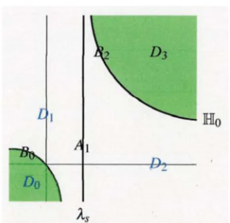
(19) 164 0 and 2n are resonances and in the case of n\geq 5 these are eigenvalues. Then the proof is completed. qed. r(2n) (\lambda_{2},\mu_{2}) Figure 8: Crossing points of hyperbolas. 4.2. Case of n=1. In this case, the asymptote of \overline{\mathb {H} _{0} is (\lambda_{\infty}(0),\mu_{\infty}(0))=(1,1) , and \lambda_{c} is not defined. \lambda_{s}=1=\lambda_{\infty}(0) . Then we have 4 sets D_{0}=G_{0},D_{1}=G_{1}\cap \mathfrak{S}_{-},D_{2}=G_{1}\cap A_{1} and D_{3}=G_{2} . The boundaries of these sets define disjoint three curves:B_{0}=\beta_{l}, B_{2}=\beta_{r} and A_{1}=\beta_{s}.. Let. n=1 .. We also see that. Table 2: Spectrum of H_{\lambda\mu} for (\lambda,\mu) on D_{k} and the edges of D_{k} for. n=1. Now we formulate next result for n=1. Theorem 4.4 Let n=1.. (1) Assume (\lambda,\mu)\in D_{k}, k\in\{0,1,2,3\} . Then H_{\lambda\mu} has k eigenvalues in (\infty,0) . In addition 0 is neither a threshold resonance and a threshold eigenvalue.. (2) Assume that (\lambda,\mu) with \lambda=\lambda_{s}=1 . Then. 0. is a super‐threshold resonance.. (3) Assume that (\lambda,\mu) in B_{k} orAı. Then results in Table 4.2 are true: In particular H_{\lambda\mu} has neither a threshold resonance nor a threshotd eigenvalue.. Proof: The theorem follows from Lemmas 2.6, 2.9, 3.3. 2.15 and 3.6.. qed. Acknowledgements This work is financially supported by Grant‐in‐Aid for Science Re‐. search (B\rangle 16H03942 from JSPS. We thank kind hospitality of Euler International Mathemat‐. ical Institute, @t. Petersburg, Russia, and E.Korotyaev for organizing “2nd Summer School: Various aspects of mathematical physics” held in July 8‐11, 2017, where this work is partial done. We also thank J. M\emptyset \mathbb{I}er, Y. Nomura and H. Morioka to send us attention of Theo‐. rem 4.3. Finally we thank Tomoko Eto for drawming beautiful Figures ı‐8..
(20) 165. \mathb {H}_{0}. \lambda_{s} Figure 9: Hyperbola for. n=1. References [1] A. Albeverio, S.N. Lakaev, K.A. Makarov, and Z.I. Muminov. The threshold effects for. the two‐particle Hamiltonians on lattices. Commun. Math. Phys., 262:91−115, 2006. [2] F. Hiroshima, Z.I, Muminov, and U. Kuljanov. Threshold of discrete Schrödinger op‐. erators with delta potentials on n ‐dimensional lattice. to appear in LinearAlgebra and. Applications.. [3] F. Hiroshima, I. Sasaki, T. Shirai, and A. Suzuki. Note on the spectrum of discrete Schrödinger operators. J.Math‐for‐lndustry, 4:105−108, 2012.. [41 H. Isozaki and H. Morioka. A Rellich type theorem for discrete Schroedinger operators. arXiv:1208.4428, preprint, 2012. [5] S.N. Lakaev and I.N. Bozorov. The number of bound states of one particıe Hamiltonian on a three‐dimensional lattice. Theoretical and Mathematical physics, 158:360−376, 2009.. [6] B. Simon. Trace ideals and their applications, 2nd ed, Amer. Math. Soc., 2005..
(21)
図
+3
関連したドキュメント
Eskandani, “Stability of a mixed additive and cubic functional equation in quasi- Banach spaces,” Journal of Mathematical Analysis and Applications, vol.. Eshaghi Gordji, “Stability
The angular velocity decreases with increasing the material parameter, the slip parameter, the buoyancy parameter, and the heat generation parameter, while it increases with
We then compute the cyclic spectrum of any finitely generated Boolean flow. We define when a sheaf of Boolean flows can be regarded as cyclic and find necessary conditions
The method employed to prove indecomposability of the elements of the Martin boundary of the Young lattice can not be applied to Young-Fibonacci lattice, since the K 0 -functor ring
Keywords and Phrases: moduli of vector bundles on curves, modular compactification, general linear
She reviews the status of a number of interrelated problems on diameters of graphs, including: (i) degree/diameter problem, (ii) order/degree problem, (iii) given n, D, D 0 ,
It is suggested by our method that most of the quadratic algebras for all St¨ ackel equivalence classes of 3D second order quantum superintegrable systems on conformally flat
We show that a discrete fixed point theorem of Eilenberg is equivalent to the restriction of the contraction principle to the class of non-Archimedean bounded metric spaces.. We
