Quantum Simulation of Interaction between Atom and Light (Mathematical Aspects of Quantum Fields and Related Topics)

全文

(1)177. Quantum Simulation of Interaction between Atom and Light Masao Hirokawa. (Hiroshima University) 1. Introduction. At the dawn of the 21st century, the solid‐state analogue of the interaction between atom and light in a superconducting circuit was theoretically proposed by Yu. Makhilin, G. Schon, and. A. Shnirman [Rev. Mod. Phys. 73, 357 (2001)] and by F. Marquardt and C. Bruder [Phys. Rev. B63, 054514 (2001) ] . It has been experimentally demonstrated by I. Chiorescu, et al. [Nature 431, 159 (2004)] and by A. Wallraff, et al. [Nature 431, 162 (2004)]. In that solid‐state analogue, an artificial atom and a microwave are used respectively for the atom and the light. The artificial atom is made by using a superconducting LC circuit. The harmonic oscillator. atom is obtained in the case without any Josephson junction as in Fig.l(a), and the 2‐ıevel atom is based on the anharmonicity coming from Josephson junctions as in Fig. 1(b). Quantizing. uperconducting\downar ow gap (a). arowarow\lrcorner [. \mu. \bullet_{-\sim}:. rcon-\dodwnuarocw_{q,.ub_{\dot{1g}ta\ldpotsO_{1^i} {\bulet}\bulet.' \dot{u}ng. :. (b). Figure 1: Superconducting LC circuit. (a) The superconducting LC circuit with no Josephson junction and its energy. spectra. (b) The superconducting LC circuit with a Josephson junction and its energy spectra.. the standing wave in the microwave resonator, we obtain its 1‐mode photon. The interaction between the artificial atom and the 1‐mode photon is made near a microwave resonator on a superconducting circuit as in Fig.2. Their most recent cutting‐edge technology is beginning to. FigUre 2: How to make the interaction between the artificiaı atom and the 1‐mode photon of the microwave resonator.. show us the ultra‐strong coupling regime or the deep‐strong coupling regime of the atom‐light. interaction beyond its standard regime of quantum electrodynamics (QED), which is even equal.

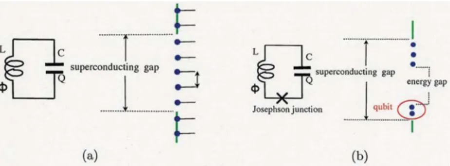
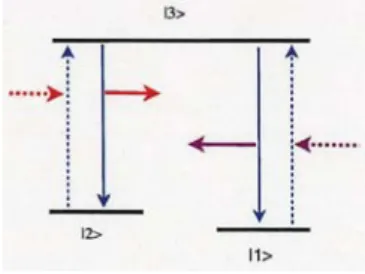
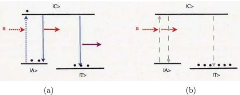
(2) 178 to that of quantum chromodynamics (QCD). For instance, more than 10% atom‐light interaction has been demonstrated in the experiment by F. Yoshihara, et al. [Nature Phys. 13, 44 (2017)]. In this paper, I introduce the following subjects on quantum simulation using the artificial atom on the superconducting circuit:. 1) the duality between a dark state and a quasi‐dark state in a cavity optomechanics as in Fig.8;. 2) the dressed photon and the Schrödinger‐cat‐like entangled ground state of the generalized quantum Rabi model;. 3) the possibility of the conversion from virtual photon to real photon in a ground state of that model.. Our purpose is in the following. Cavity QED, which describes the interaction between the atom and the 1‐mode photon in the cavity, can be demonstrated on a superconducting cir‐ cuit. That cavity QED demonstrated on superconducting circuits is called circuit QED. The leading edge of technology in circuit QED has been enabling us to demonstrate the interaction between atom and light with superconducting circuits. In addition, the current technology of the mechanical resonators lately supplies us with mechanical phonon. The mechanical phonon can be simulated by a superconducting circuit. Therefore, our goal is the quantum simulation of the atom‐light interaction, and moreover, of the atom‐light system coupled with phonon on superconducting circuits. For our quantum simuıation, we make the foılowing replacements: We. replace a true atom with a superconducting LC circuit with or without Josephson junction(s). Here, a 2‐level atom is demonstrated by the superconducting LC circuit with some Josephson junctions. Photon is given by the quantization of the microwave in a cavity. We can replace the 1‐mode photon with a superconducting LC circuit because a photon as well as a phonon is a boson. As for phonon, we are interested in the mechanical phonon made by giving an artificial vibration to the cavity and considering its quantization. We can also replace the 1‐mode phonon with a superconducting LC circuit.. 2. Dark State and Quasi‐Dark State & A Duality between Them. The electromagnetically induced transparency (EIT) is a physical phenomenon in quantum op‐ tics. Usually, to obtain EIT we prepare the so‐caıled. A ‐shaped. 3‐level system as in Fig.3. We. 13>. ì. Figure 3: The \Lambda‐shaped 3‐level system.. continue irradiating the 3‐level system with the laser ‘a’ like Fig.4(a). Time enough passes, and there is neither any photon in the state |A\rangle nor in the state |C } as in Fig.4(b). Thus, even if we irradiate the A‐shaped 3‐level system with the laser ‘a’, the laser goes through the system because neither absorption nor emission takes place. This is EIT. In this EIT, although the state |T\} is an excited state, it cannot emit the light because it does not have any photon. We call. the state |T} a dark state..

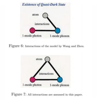
(3) 179 1G. 1. 1. a. a. t e\cdot\cdot\triangleright 1...J..〉. *. \overline{W>}. 1A 〉. 1. 1. 1. 1. 1. \underline{1\downar ow}1b. \frac{o\cdot\foral \cdot eo1}{W\geq}. (a). (b). Figure 4: (a) Irradiation of the ıaser a to the 3‐ıeveı system. (b) EIT and the dark state.. We should mention the possibility of dark state for the qubit coupled to light. We remember a qubit is a 2‐level system. However, Emary points out the possibility of the existence of a. dark state even for the 2‐level system [J. Phys.. B:. At. Mol. Opt. Phys. 46, 224008 (2013)].. Moreover, Zhu and other collaborators succeeded in demonstrating it in their experiment [Nature Comm. 5, 3424 (2014)]. More precisely, they experimentally demonstrated a dark state for the superconducting qubit coupled with the NV centers in diamond. Theoretically to explain their dark state, they model a spin ensemble of NV centers as a number of harmonic oscillators, and they employ a simple modeı mathematically regarded as describing a 2‐level atom coupled with a 1‐mode photon and another 1‐mode boson, We think of the another boson as a phonon in this paper. In their model, there is no interaction between the 2‐level atom and the 1‐mode phonon. (Fig.5). Existence ofDark State. l‐m. onon. Figure 5: Interactions of the model by Zhu. e\ell lJl.. Meanwhile, Wang and Zhou consider an atom‐cavity system surrounded by a heat bath, where their atom‐cavity system is the 2‐level atom coupled with the 1‐mode photon. They found a notion of quasi‐dark state, which results from the two couplings, that is, the coupling between the atom and the heat bath, and the coupling between the 1‐mode photon and the heat bath. Their heat bath is regarded as a 1‐mode phonon in this paper. They show that the. quasi‐dark state appears when the atom‐ıight coupling is absent (Fig.6). In the two models, the notions of dark sate and quasi‐dark state are antipodes to each other: The model used by Zhu et al. has no interaction between the 2‐level atom and the 1‐mode. phonon (Fig.5), and thus, any quasi‐dark state does not appear. Wang and Zhou’s model has no interaction between the 2‐ıevel atom and the 1‐mode photon (Fig.6), and thus, any dark state does not appear. A question arises then. Can each of a dark state and a quasi‐dark state have individual chance to appear if both interactions, between the 2‐level atom and the 1‐mode. photon, and between the 2‐level atom and the 1‐mode phonon, exist (Fig.7)? To consider this problem, we imagine a set‐up in cavity optomechanics. We give an artificial vibration to our cavity as in Fig.8. This vibration changes the length of the resonator, and thus, the wave ıength of the standing wave in the resonator also changes. This change of the wave length makes the.

(4) 180 Existence ofQuasi‐Dark State. l‐m. onon. Figure 6: Interactions of the moclel by Wang and Zhou.. l‐m. onon. Figure 7: All interactions are assumed in this paper.. interaction between the 1‐mode photon and the 1‐mode phonon considering their quantization. creation of. Figure 8: Cavity‐optomechanicaı system.. We make the mathematical set‐ups now. The atom‐cavity Hamiltonian describing the atom coupled with the 1‐mode photon is given by. H_{cav} :=\omega_{a}a^{\dag er}a+\omega_{b}b^{\dag er}b+(\lambda^{*\dag er}ab+ \lambda b^{\dag er}a). ,. where a and a\dag er are respectively the annihilation and crea ion operators of an atom, b and b\dag er are respectively the annihilation and creation operators of the 1‐mode photon in a cavity. \lambda denotes the strength of the atom‐cavity interaction. In Ref.[1], the two cases are considered: a and a\dag er are. the annihilation and creation operators of 1) a quantum harmonic oscillator and 2) a spin. In this paper, we consider the latter case onıy. That is, the case where the atom is the so‐called 2‐level atom. In this case, the Hamiltonian H_{cav} is that of the Jaynes‐Cummings model: H_{cav}=H_{JC}, where. H_{JC}:=\omega_{a}\sigma_{+}\sigma_{-}+\omega_{b}b^{\dag er}b+(\lambda^{*} \sigma+b+\lambda b^{\dag er}\sigma_{-}). ,. and the annihilation and creation operators, a and a\dagger , are respectively the spin annihilation and creation operators, a=\sigma_{-}\equiv(\sigma_{x}-i\sigma_{y})/2 and a\dagger=\sigma+\equiv(\sigma_{x}+i\sigma_{y})/2 . We use standard.

(5) 181 181. notations for the Pauli matrices throughout this paper:. \sigma_{x}:=(\begin{ar ay}{l } 0 1 1 0 \end{ar ay}), \sigma_{y}:=(\begin{ar ay}{l } 0 -\dot{i} i 0 \end{ar ay}), \sigma_{z}:=(\begin{ar ay}{l } 1 0 0 -1 \end{ar ay}). We apply a phonon field to the atom‐cavity system so that the total Hamiltonian. H :=H_{cav}+\omega_{c}c^{\dagger}c+(\xi^{*}a^{\dagger}c+\xi c^{\dagger}a)+ (\kappa^{*}b^{\dagger}c+\kappa c^{\dagger}b). H. becomes. ,. where c and c\dag er are respectively the annihilation and creation operators of the 1‐mode phonon. \xi is the coupıing constant of the atom and the 1‐mode phonon, and \kappa the coupling constant of the 1‐mode photon and the 1‐mode phonon. We respectively denote the ground and excited spin‐states by |g\}_{a} and |e\}_{a} . We denote the Fock state by |n\rangle_{\#}, \#=b, c;n=0,1,2, , where n is the number of photons for \#=b , and the number of phonons for \#=c . The ground state of H is obviously |g\rangle_{a}|0)_{b}|0\rangle_{c} . We assume the following condition: \cdots. \omega=\omega_{b}=\omega_{c}.. First, we explain the dark state that Zhu et al. found and the quasi‐dark state that Wang and Zhou found. We consider the case without interaction between the atom and the 1‐mode. phonon, i.e., \xi=0 . As shown in Ref.[1], an excited eigenstate with the eigenenergy. \omega. is obtained. as. | \mathcal{D}\}=\frac{\kap a}{\sqrt{\kap a^{2}+\lambda^{2} |e\rangle_{a}|0\} _{b}|0\}_{c}-\frac{\lambda}{\sqrt{\kap a^{2}+\lambda^{2} |g\}_{a}|0\}_{b}|1) _{c}.. This is the dark state that Zhu et al. found. On the other hand, we consider the case without. interaction between the atom and the 1‐mode photon, i.e., eigenstate with the eigenenergy. \omega. \lambda=0 .. As shown in Ref.[1], an excited. is obtained as. | \overline{\mathcal{D} \rangle=\frac{\kap a}{\sqrt{\kap a^{2}+\xi^{2} |e\rangle_{a}|0\}_{b}|0\}_{c}-\frac{\xi}{\sqrt{\kap a^{2}+\xi^{2} |g\rangle_{a} |1)_{b}|0\rangle_{c}. This is the quasi‐dark state that Wang and Zhou found. Now, we consider the case where both interactions exist, i.e., \lambda\xi\neq 0 . We define the two functions:. E(x, y):= \omega-\kappa\frac{y}{x}. and. f(x, y):=(\begin{ar ay}{l} \kappa x - x\kappa \end{ar ay})y.. As shown in Ref.[1], we have the following duality:. (a) If f(\lambda, \xi)=\omega-\omega_{a} , then there is a dark state |\mathcal{D}\rangle with the eigenvalue E(\lambda, \xi) . (b) If f(\xi, \lambda)=\omega-\omega_{a} , then there is a quasi‐dark state. |\overline{\mathcal{D}\rangle with the eigenvalue E(\xi, \lambda) .. Here,. and. | \mathcal{D}\rangle=\frac{\kap a}{\sqrt{\kap a^{2}+\lambda^{2} |e\}_{a}|0\} _{b}|0\rangle_{c}-\frac{\lambda}{\sqrt{\kap a^{2}+\lambda^{2} |g\rangle_{a} |0\rangle_{b}|1\}_{c}. | \overline{\mathcal{D} \rangle=\frac{\kap a}{\sqrt{\kap a^{2}+\xi^{2} |e\rangle_{a}|0\}_{b}|0\rangle_{c}-\frac{\xi}{\sqrt{\kap a^{2}+\xi^{2} |g\}_{a} |1\rangle_{b}|0\}_{c}.. In addition to this duality, we have a duality for particle numbers: For \{b\dagger b\}_{(\lambda,\xi)} , the dark‐ state expectation of light, and \{c\dag er c\rangle_{(\lambda,\xi)} , the quasi‐dark‐state expectation of phonon, defined. by. { b^{\dag er}b\rangle_{(\lambda,\xi)} :=\langle \mathcal{D}|b^{\dag er}b|\mathcal{D}\rangle and. \{c^{\dag er}c\rangle_{(\xi,\lambda)} :=\langle\overline{\mathcal{D} |c^{\dag er}c|\overline{\mathcal{D} \rangle,. we obtain. \{b\dag er b\rangle_{(\lambda,\xi)}=\langle c^{\dag er}c\}_{(\xi,\lambda)} (See Ref.[1]). Moreover, we can show the necessity of \kappa\neq 0 , i.e., an interaction between the 1‐mode photon and the 1‐mode phonon, to obtain the chance that each of a dark state and a quasi‐dark state exists in the case \lambda\xi\neq 0 (See Ref.[1])..

(6) 182 3. Dressed Photon and the Schrödinger‐Cat‐Like Entangled Ground State of the Generalized Quantum Rabi Model. We express the spin state in the following:. |\upar ow\rangle. :=(\begin{ar y}{l 1 0 \end{ar y}). \in \mathbb{C}^{2}. and. |\downar ow\rangle. :=(\begin{ar y}{l 0 1 \end{ar y}). \in \mathbb{C}^{2}.. In this section, we denote by a and a\dagger the annihiıation and creation operators of 1‐mode photon, respectively. The generalized quantum Rabi Hamiltonian is given by. H( \omega_{a},\omega_{c}, g):=\frac{\hslash}{2}(\omega_{a}\sigma_{z}- \varepsilon\sigma_{x})+\hslash\omega_{c}(a^{\dag er}a+\frac{1}{2})+\hslash g\sigma_{x}(a+a\dag er) then. Here, \omega_{a} is the transition frequency of a 2‐level atom demonstrated by a superconducting circuit, \varepsilon the bias energy parameter of the superconducting circuit, \omega_{c} the frequency of the 1‐ mode photon in a cavity on the superconducting circuit, and g the coupling strength between the atom and 1‐mode photon. The Hamiltonian \mathcal{H}_{tota1} that Yoshihara et al. considered to explain their experimental results. [Nature Phys. 1344 (2017)] is. \mathcal{H}_{tota{\imath}}:=U_{xz}H(w_{a}, \omega_{c}, g)U_{xz}^{*}, where. U_{xz}:= \frac{1}{\sqrt{2} (\begin{ar ay}{l} 1 1 -1 1 \end{ar ay}). .. We can show that, in the case \varepsilon=0 , the ground state \psi_{g} of their total Hamiltonian \mathcal{H}_{tota1} is welı approximated by the entanglement between the two coherent states for sufficiently large coupling constants, and makes a Schrödinger‐cat‐like entangled state:. \psi_{g} \ap rox \frac{e^{-g^{2}/2\omega_{c}^{2} {\sqrt{2} \sum_{n=0} ^{\infty}\{\frac{(-g/\omega_{c})^{n} {\sqrt{n!} |\upar ow, n\rangle+ \frac{(g/\omega_{c})^{n} {\sqrt{n!} |\downar ow, n\}\}, g\g 1. This results from the mathematical result that the Hamiltonian \mathcal{H}_{tota{\imath} converges to that for the. Schrödinger‐cat‐like entangled state as. 4. garrow\infty. in the norm resolvent sense (See Ref.[2]).. Possibility of Conversion from Virtual Photon to Real Photon in Ground State of the Generalized Quantum Rabi Model. Moore theoretically proposed the so‐called dynamical Casimir effect [J. Math. Phys. 11, 2679 (1970)]. C. M. Wilson, et al. succeeded in demonstrating the dynamical Casimir effect in their experiment using a superconducting circuit [Nature 479, 376 (2011)]. Namely, they succeeded in deriving a real photon from the vacuum fluctuation caused by virtual photons. In this section, we argue a possibility of the conversion from virtual photon to real photon in the ground state of the generalized quantum Rabi model. We consider the Hamiltonian with A^{2} ‐term. We define. the Hamiltonian with the A^{2} ‐term by. H_{A^{2} :=H(\omega_{a}, \omega_{c}, g)+\hslash C_{g}g(a+a^{\dagger})^{2} where C_{g} is a function of the coupling strength C.. g. given as C_{g}=Cg or. C_{g}=Cg^{2}. with a constant. Since we have to mind and cope with the effect coming from the A^{2} ‐term (i.e., the quadratic coupling), we follow the pair theory explained in Henley and Thirring’s textbook [“Elementary.

(7) 183 Quantum Field Theory” (New York: McGraw‐Hilı) 1962]. We remember the following physical fats: The ‘virtual photon’ is a technical term in the theory of elementary particle. It is the gauge particle causing the Coulomb force. Any virtual photon cannot directly be observed. We denote by |E_{v} }, \nu=0,1,2, , the eigenstates of the total Hamiltonian H_{A^{2}} , and by E_{\nu} the corresponding eigenenergies with E_{0}\leq E_{1}\leq E_{2}\leq The ground‐state expectation of bare photon defined by \cdots. N_{0}^{bare}:=\{E_{0}|a^{\dagger}a|E_{0}\}. is for the bare photons, and includes the number of virtuaı photons as weıl as that of reaı ones. Let \triangle\Phi be the fluctuation for the bare‐photon field \Phi=(a+a\dagger)/\sqrt{2\omega_{c}} at the ground state |E_{0}\rangle, i.e.,. \triangle\Phi=\sqrt{\langle E_{0}|(\Phi-\{E_{0}|\Phi|E_{0}\})^{2}|E_{0}\}}. As shown in Ref.[2], we have the followings:. (a). (\triangle\Phi)^{2}\leq(2N_{0}^{bare}+1)/\omega_{C}.. (b). \lim_{garrow\infty}N_{0}^{bare}=\infty.. Inequality (a) says that the number of bare photons increases if the fluctuation grows larger and larger. Thus, the number of virtual photons increases as well. We follow the pair theory to avoid this increase in the number of virtual photons. The new annihilation and creation operators, b and b\dag er , for real photons are introduced so that the reıations,. a=M_{1}b+M_{2}b^{\dagger}. and. a\dagger=M_{2}b+M_{1}b^{\dagger},. are satisfied, where. M_{1}=\frac{1}{2}\{ sqrt{\frac{\omega_{c} {\omega_{g} +\sqrt{\frac{\omega_{g} }{\omega_{c} \}. and. M_{2}=\frac{1}{2}\{ sqrt{\frac{\omega_{c} {\omega_{g} -\sqrt{\frac{\omega_{g} }{\omega_{c} \}.. Then, we can obtain the so‐called Hopfield‐Bogoliubov transformation (See Ref.[2]): For arbi‐ trary \omega_{c}, g, C_{g} , the Hopfield‐Bogoıiubov transformation U is unitary so that U^{*}H_{A^{2}}U=H(\omega_{a}, \omega_{g},\overline{g}). ,. where. \omega_{g}=\sqrt{\omega_{c}^{2}+4C_{g}g\omega_{c}. and. \tilde{g}=g\sqrt{\frac{\omega_{c}{\omega_{g} .. We here note that the Hopfield‐Bogoliubov transformation is unitary for our model without any restriction.. Thanks to the unitarity of the Hopfield‐Bogoliubov transformation, we can define the nor‐ malized eigenstates of the renormalized Hamiltonian H(\omega_{a}, \omega_{g},\overline{g}) with the A^{2} ‐term effect by. |E_{\nu}^{ren}\}:=U^{*}|E_{\nu}\}, and then, the eigenenergy E_{\nu}^{ren} of each eigenstate |E_{\nu}^{ren} } is, of course, E_{\nu} . We can show that E_{0} is always less than E_{1} , i.e., E_{0}<E_{1} . We consider the renormalized ground‐state expectation of real photon,. N_{0}^{ren}:=\{E_{0}^{ren}|a\dagger a|E_{0}^{ren}\},. and how the ground state of the renormaıized quantum Rabi Hamiltonian has a real photon.. As shown in Ref.[2], we have the following estimates:. L^{ren}( g)^{2}\leq N_{0}^{ren}\leq\frac{\overline{g}^{2} {\omega_{g}^{2} = \omega_{c}^{-1/2}(\frac{\omega_{c} {g^{4/3} +\frac{4C_{g} {g^{1/3} )^{-3/2} \vec{gar ow\infty}0,.

(8) 184 provided that the function L^{ren}(g) satisfies L^{ren}(g)\geq 0 , where. L^{ren}(g):=\frac{\overline{g}{\omega_{g}-\sqrt{\frac{\sqrt{\omega_{a}^{2}+ \varepsilon^{2}(1-e^{-2\overline{g}^{2}/\omega_{g}^{2}){2\omega_{g} . We show the upper bound and the lower bound in Fig.9. Then, Fig.9 says that the ground. g s^{\Rightarow}. \hat{=\vee S} 2 2 \underline{\S*}. 1. I. \tilde{S}. \hat{-\vee\varepsilon} 0 0 § strength g of interaction. \frac{\S}B 3. \hat{wedg=\ve }. \underlin{\xi:}. 2. 5. 1. 5. strength. C_{l}4.5xg.\omega_{a}4. \omega_{c}=0.75. I.. BR\Leftrighaow\infty 3. -. |^{-}. 2 --1!|. C_{S}4.5xg^{-}. g. of interaction. . tu,t.1, (0,t.7S. \hat{frcv\Rightarow}{\h ve} 2 \underlin{o*:}. 2.5. 1.5. \s\dot{\S} im_{E}\wedge\ap rox\ve \over0_{0} line{\sim} 0.51 - 1 -!21|- \ha4t{\frac6{} \ve88} \10 overline{*} 0\S .51 0_{0} 2 4 6 8 10. Figure 9: N_{0}^{ron} sits bet_{\mathbb{R}A_{-}1}IkPlBRb\iotalffi The upper line\Rightar ow denotes the \mathfrak{W}w1\mathfrak{W}I\eta A_{C}fl\vartheta\alpha ihe lower line is the lower bound.. state is almost a vacuum and we can expect no reaı photon for large constant C (see the case C=0.5) . However, we can expect one or two real photon(s) for sufficiently small C (see the case C=0.05 ). Thus, we are interested in where the real photon comes from. We denote the spin‐chiraı. transformed state, \sigma_{x}|E\rangle , by |\overline{E}\rangle :=\sigma_{x}|E }. Then, actually, the sate |\overline{E}\rangle becomes a spin‐chiraı st ate, in a sense, on the surface on the spin‐chiral mirror. For more details, see Ref.[2]. As given in Ref.[2], we obtain the following expression: For any coupling constant g (c). N_{0}^{ren}=|\{ overline{E}_{0}^{ren}|E_{0}^{ren}\|^{2}\frac{\overline{g}^{2} {\omega_{g}^{2}+\hsla h^{2}\overline{g}^{2}\sum_{\nu=1}^{\infty} \frac{|\ overline{E}_{\nu}^{ren}|E_{0}^{ren}\|^{2}{(E_{\nu}-E_{0}+ \hsla h\omega_{g})^{2}.. (d) There is an. \nu_{*}. so that. 0<\hslash^{2}\overline{g}^{2}\frac{|\langle\overline{E}_{\nu_{*}^{ren}|E_{0}^ {ren}\|^{2}{(E_{\nu_{*}-E_{0}+\hslash\omega_{g})^{2}\leqN_{0}^{ren}. Expression (c) says that the real photon comes from the spin‐chiral states to the ground state. Similarly, we have the following:. (e) For sufficientıy small. C,. the ground‐state expectation of bare photons is expressed as. N_{0}^{bare}=|\{ overline{E}_{0}|E_{0}\|^{2}\frac{g^{2}{\omega_{c}^{2}+ \hslash^{2}g^{2}\sum_{\nu=1}^{\infty}\frac{|\langle\overline{E}_{\nu}|E_{0} \rangle|^{2}{(E_{l/}-E_{0}+\hslash\omega_{c})^{2}..

(9) 185 5. Summary. In this paper, we have showed the following results:. 1. the duality between a dark state and a quasi‐dark state for an artificial atom coupled to both the 1‐mode photon and 1‐mode phonon in cavity optomechanics; 2. the dressed photon and the Schrödinger‐cat‐like entangled ground state of the generalized quantum Rabi model;. 3. the possibility of the conversion from virtual photon to real photon in a ground state of that model.. Concerning 1, we are considering a design of the superconducting circuit experimentally to demonstrate the duality. The dark state is expected to be used as a quantum memory, and therefore, the duality could be useful for exchanging the two quantum memories. Regarding 3, we are proposing the method of how to derive the real photon in the ground state in circuit QED. The ground state is the bound state with the lowest energy, and thus, it is stable. So, the real photon in a ground state means the stable storage of a photon. Therefore, if we can succeed in obtaining a technology to derive the real photon, we have the technology for stably saving and drawing a photon from the ground‐state bank.. Acknowledgments The author acknowledges the support from JSPS Grant‐in‐Aid for Scientific Researches (B) 26310210 and (C) 26400117. References. [1] M. Hirokawa, Duality between A Dark State And A Quasi‐Dark State, Annals of Physics (N.Y.) 377: 229‐242 (2017). [2] M. Hirokawa, J. M \emptyset ıler, and I. Sasaki, A Mathematical Analysis of Dressed Photon in Ground State of Generalized Quantum Rabi Model Using Pair Theory, Journal of Physics. A: Mathematical and Theoretical 50: 184003 [20pages] (2017)..

(10)