"High-dimensional Motion Segmentation by Variational Autoencoder and Gaussian Processes"

High-dimensional Motion Segmentation by

Variational Autoencoder and Gaussian Processes

Masatoshi Nagano

, Tomoaki Nakamura

, Takayuki Nagai

, Daichi Mochihashi

,

Ichiro Kobayashi

and Wataru Takano

Abstract— Humans perceive continuous high-dimensional

in-formation by dividing it into significant segments such as words and units of motion. We believe that such unsupervised segmentation is also important for robots to learn topics such as language and motion. To this end, we previously proposed a hierarchical Dirichlet process–Gaussian process– hidden semi-Markov model (HDP-GP-HSMM). However, an important drawback to this model is that it cannot divide high-dimensional time-series data. Further, low-high-dimensional features must be extracted in advance. Segmentation largely depends on the design of features, and it is difficult to design effective features, especially in the case of high-dimensional data. To overcome this problem, this paper proposes a hierarchical Dirichlet process–variational autoencoder–Gaussian process– hidden semi-Markov model (HVGH). The parameters of the proposed HVGH are estimated through a mutual learning loop of the variational autoencoder and our previously pro-posed HDP-GP-HSMM. Hence, HVGH can extract features from high-dimensional time-series data, while simultaneously dividing it into segments in an unsupervised manner. In an experiment, we used various motion-capture data to show that our proposed model estimates the correct number of classes and more accurate segments than baseline methods. Moreover, we show that the proposed method can learn latent space suitable for segmentation.

I. INTRODUCTION

Humans perceive continuous high-dimensional informa-tion by dividing it into significant segments such as words and units of motion. For example, we recognize words by segmenting speech waves, and we perceive particular motions by segmenting continuous motion. Humans learn words and motions by appropriately segmenting continuous information without explicit segmentation points. We believe that such unsupervised segmentation is also important for robots, in order for them to learn language and motion.

To this end, we previously proposed a hierarchical Dirich-let process–Gaussian process–hidden semi-Markov model (HDP-GP-HSMM) [1]. HDP-GP-HSMM is a nonparametric Bayesian model that is a hidden semi-Markov model whose emission distributions are Gaussian processes, making it possible to segment time-series data in an unsupervised

1_{Department of Mechanical Engineering and Intelligent Systems, The}

University of Electro-Communications, Chofu-shi, Japan

2_{Department of Systems Innovation, Osaka University, Toyonaka-shi,}

Japan

3_{Department of Mathematical Analysis and Statistical Inference, Institute}

of Statistical Mathematics, Tachikawa, Japan

4_{Department of Information Sciences, Faculty of Sciences, Ochanomizu}

University, Bunkyo-ku, Japan

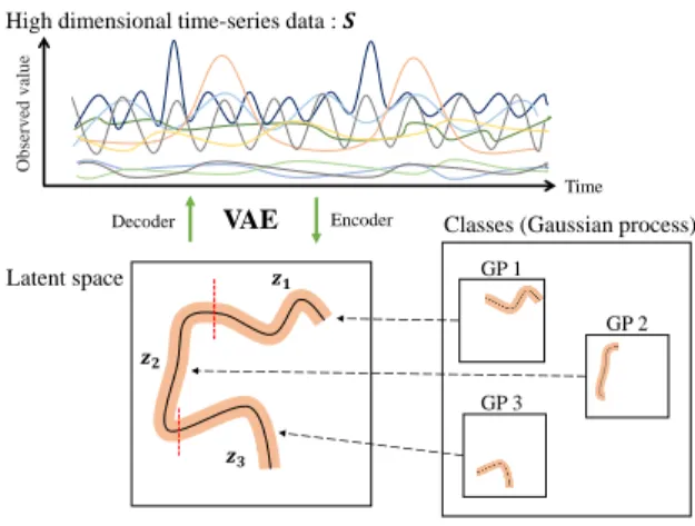
Correspondence∗:[email protected] Time Ob serv ed v alu e

High dimensional time-series data : 𝑺

VAE Encoder Decoder

Latent space

Classes (Gaussian process)

GP 1 GP 2 GP 3 𝒛𝟏 𝒛𝟐 𝒛𝟑

Fig. 1. Overview of the generative process of the HVGH.

manner. In this model, segments are continuously represented using a Gaussian process. Moreover, the number of seg-mented classes can be estimated using hierarchical Dirichlet processes [2]. The Dirichlet processes assume an infinite number of classes. However, only a finite number of classes are actually used. This is accomplished by stochastically truncating the number of classes using a slice sampler [3].

However, our HDP-GP-HSMM cannot deal with high-dimensional data, and feature extraction is needed in order to reduce the dimensionality in advance. Indeed, segmentation largely depends on this feature extraction, and it is difficult to extract effective features, especially in the case of high-dimensional data. To overcome this problem, this paper introduces a variational autoencoder (VAE) [4] to the HDP-GP-HSMM. Thus, the model we propose in this paper is a hierarchical Dirichlet process–variational autoencoder– Gaussian process–hidden semi-Markov model (HVGH). Fig. 1 shows an overview of HVGH. The observation sequence is compressed and converted into a latent variable sequence by the VAE, and the latent variable sequence is divided into segments by HDP-GP-HSMM. Furthermore, parameters learned by HDP-GP-HSMM are used as the hyperparameters for the VAE. In this way, the parameters are optimized in a mutual learning loop, and appropriate latent space for segmentation can be learned by the VAE. In experiments, we evaluated the efficiency of the proposed HVGH using real motion-capture datasets. The experimental results show that HVGH achieves more accuracy than baseline methods. Many studies on unsupervised motion segmentation have been conducted. However, heuristic assumptions are used in

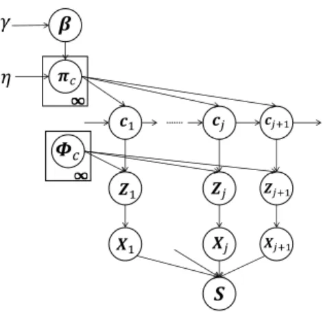
𝜂 𝜱𝑐 𝒁1 𝒁𝑗 𝒁𝑗+1 𝑿1 𝑿𝑗 𝑿𝑗+1 𝝅𝑐 𝜷 𝒄1 𝒄𝑗 𝒄𝑗+1 𝛾 𝑺 Fig. 2. Graphical model of HVGH.

many of them [5], [6], [7]. Moreover, some methods use motion features such as the zero velocity of joint angles [8], [9], [10]. However, this assumption usually leads to over-segmentation [6].

Furthermore, studies have proposed methods of detecting change points in time-series data in an unsupervised manner [11], [12], [13], [14]. These are the methods of finding points with different fluctuations based on previous observations. However, change points do not necessarily indicate the boundary of segments.

In some studies, segmentation is formulated stochastically using hidden Markov models (HMMs) [15], [16], [17], [18]. However, it is difficult for HMMs to represent complicated motion patterns. Instead, we use Gaussian processes, a type of non-parametric model that can better represent compli-cated time-series data compared to HMMs. We confirmed that our GP-based model can estimate segments more accu-rately than HMM-based methods [1].

In some studies, the number of classes is estimated by introducing a hierarchical Dirichlet process (HDP) into an HMM [15], [19]. An HDP is a method of estimating the number of classes by assuming an infinite number of classes. Fox et al. extended an HDP–HMM to make a so-called sticky HDP-HMM, which prevents over-segmentation by increasing the self-transition probability [19].

Among methods of combining probabilistic models with neural networks, a method of classifying complicated data using a GMM and VAE was proposed [20]. By contrast, our proposed HVGH is a model that combines a probabilistic model with VAE for segmenting high-dimensional time-series data.

II. HIERARCHICALDIRICHLETPROCESS–VARIATIONAL AUTOENCODER–GAUSSIANPROCESS–HIDDEN

SEMI-MARKOVMODEL(HVGH)

Fig. 2 shows a graphical model of our proposed HVGH, which is a generative model of time-series data. In this model, cj(j = 1, 2,· · · , ∞) denotes the classes of the

segments, where the number of classes is assumed to be countably infinite. Probability πcdenotes the transition

prob-ability, which is generated from the the Dirichlet process

is parameterized by β, and the β is generated by the GEM distribution—with the so-called stick-breaking process (SBP):

β ∼ GEM(γ), (1)

πc ∼ DP(η, β). (2)

The class cj of the j-th segment is determined by the class

of the (j− 1)-th segment and transition probability πc. The

segment of latent variables Zj is generated by a Gaussian

process whose parameter is ϕ_c, as follows:

cj ∼ p(c|cj−1, πc, α), (3)

Zj ∼ GP(Z|ϕcj), (4)

where ϕc denotes a set of segments of latent variables that

are classified into class c. The segment Xjis generated from

the segment of the latent variables Zj by using decoder Pdec

of the VAE:

Xj ∼ pdec(X|Zj). (5)

The observed sequence s = X0, X1,· · · , XJ is assumed

to be generated by connecting segments Xj sampled by

the above generative process. Similarly, the sequence of the latent variables ¯s = Z0, Z1,· · · , ZJ is obtained by

connecting the segments of the latent variables Zj. In this

paper, the i-th data point included in Xjis described as xji,

and the i-th data point included in Zj is described as zji.

If the characters represent what they obviously are, we omit their subscripts.

A. Hierarchical Dirichlet Processes (HDP)

In this study, the number of segment classes is estimated by utilizing a non-parametric Bayesian model. In a non-parametric Bayesian model, an infinite number of classes is assumed, and the classes are sampled from an infinite-dimensional multinomial distribution. To realize this, an infinite-dimensional multinomial distribution must be con-structed, and one of the methods for this is the SBP [3].

vk ∼ Beta(1, γ) (k = 1,· · · , ∞), (6)

βk = vk k∏−1

i=1

(1− vi) (k = 1,· · · , ∞). (7)

This process is represented as β∼ GEM(γ), where “GEM” denotes the co-authors Griffiths, Engen, and McCloskey [21]. In the case of models like the HMM, all states have to share their destination states and have different probabilities of transitioning to each state. To construct such a distribution, the distribution β generated by the SBP is shared with all states as a base measure, and transition probabilities πc,

which are different in each state c, are generated by another Dirichlet process. The method in which the probability distribution is constructed by a two-phase Dirichlet process is called an HDP.

B. Gaussian Process (GP)

In this paper, each class represents a continuous trajectory by learning the emission zi of time step i using a Gaussian

process. In the Gaussian process, given the pairs (i, ϕc) of

time step i and its emission, which are classified into class c, the predictive distribution of znew_{of time step i}new_becomes

a Gaussian distribution whose parameters are µ and σ2_:

p(znew|inew, ϕ_c, i) ∝ N (z|µ, σ2), (9) µ = kTC−1i, (10) σ2 = c− kTC−1k. (11) Here, k(·, ·) denotes the kernel function, and C is a matrix whose elements are

C(ip, iq) = k(ip, iq) + ω−1δpq, (12)

where ω denotes a hyperparameter that represents noise in the observations. k is a vector whose elements are k(ip, inew), and c is k(inew, inew). A Gaussian process can

represent complicated time-series data owing to the kernel function. In this paper, we used the following kernel function, which is generally used for Gaussian processes:

k(ip, iq) = θ0exp(−

1

2θ1||ip− iq||

2

+ θ2+ θ3ipiq), (13)

where, θ_∗ denotes the parameters of the kernel.

Additionally, if the observations are composed of multi-dimensional vectors, we assume that each dimension is in-dependently generated. Therefore, the predictive distribution GP(z|ϕc) that the emission z = (z0, z1,· · · ) of time step i

is generated by a Gaussian process of class c is computed as follows: GP(z|ϕc) = p(z0|i, ϕc,0, i) × p(z1|i, ϕc,1, i) × p(z2|i, ϕc,2, i)· · · (14) = N (z|µ0, σ02)N (z|µ1, σ12)N (z|µ2, σ22)· · · . (15) By using this probability, the latent variables can be classified into the classes. Moreover, because each dimension is inde-pendently generated, the mean vector µc(i) and the

variance-covariance matrix Σc(i) of GP(zji|Zc) are represented as

follows: µ_c(i) = (µ0, µ1, µ2,· · · ), (16) Σc(i) =    σ2 1 0 0 0 σ2 2 0 0 0 . ..    , (17) where (µ0, µ1, µ2,· · · ) and (σ02, σ 2 1, σ 2 2,· · · ) respectively

represent the mean and the variance of each dimension. HVGH is a model whereby VAE and GP influence each other mutually by using µc(i) and Σc(i) as the prior distribution

of the VAE.

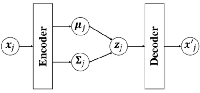
𝒙

Encoder

𝝁

𝚺

𝒛

Decoder

𝒙′

Fig. 3. Variational autoencoder (VAE).

C. Overview of the Variational Autoencoder

In this paper, we compress a high-dimensional time-series observation into low-dimensional latent variables using the VAE [4]. The VAE is a neural network that can learn the correspondence between a high-dimensional observation x and the latent variable z. Fig. 3 shows an overview of the VAE. A Gaussian distribution with a mean µenc(x)

and variance Σenc(x) that are estimated by using encoder

networks from input x is used as qenc(z):

qenc(z) =N (z|µenc(x), Σenc(x)). (18)

The latent variable z is stochastically determined by this distribution, and x′ is generated through decoder networks pdec:

z ∼ qenc(z), (19)

x′ ∼ pdec(x|z). (20)

The parameters of the encoder and decoder are determined to maximize the likelihood by using the variational Bayesian method. Generally, the prior distribution of the VAE is a Gaussian distribution whose mean is the zero vector 0, and the variance–covariance matrix is the identity matrix e. On the other hand, HVGH uses a Gaussian distribution whose parameters are µ_c(i) and Σc(i) of class c into which zji is

classified. As a result, latent space suitable for segmentation can be constructed. By using this VAE, a sequence of the observation s = X0, X1,· · · , XJ is converted to a

se-quence of the latent variables ¯s = Z0, Z1,· · · , ZJ through

the encoder.

III. PARAMETERINFERENCE

Fig. 4 shows an outline of parameter estimation for HVGH. A sequence of observations s is converted to a sequence of latent variables ¯s by the VAE. Then, by the HDP-GP-HSMM, the sequence of latent variables ¯s is di-vided into segments of latent variables Z0, Z1,· · · , and the

parameters µ_c(i) and Σc(i) of the predictive distribution of z are computed. This predictive distribution is used as a prior distribution of the VAE. Thus, the parameters of the VAE and HDP-GP-HSMM are mutually optimized.

A. Parameter Inference of HDP-GP-HSMM

The parameters of HDP-GP-HSMM are estimated in the same manner that we proposed in [1]. Here, we briefly explain the parameter inference and see [1] for detail.

Observed sequence: 𝒔

Initial parameters: 𝝁𝒄(𝑖) = 𝟎, 𝚺+(𝑖) = 𝒆

Latent variable sequence: 𝒔-Mean:𝝁.(𝑖)

Variance:𝚺.(𝑖)

- Divide 𝒔- into segments 𝒁0, 𝒁1, ⋯ by

HDP-GP-HSMM

- Update parameters 𝝁.(𝑖), 𝚺.(𝑖)

Convert 𝒔 to latent variable sequence 𝒔-by VAE using 𝝁_. 𝑖 and 𝚺_. 𝑖 as prior

Segments: 𝒁3, 𝒁1, ⋯

Classes: 𝑐₅, 𝑐₁,⋯

Fig. 4. Overview of parameter estimation for HVGH. The parameters are learned by a mutual learning loop of the VAE and HDP-GP-HSMM.

In the HDP-GP-HSMM, segments and classes of latent variables are determined by sampling. For efficient estima-tion, we utilize a blocked Gibbs sampler [22], in which all segments and their classes in one observed sequence are sampled. The segments of latent variables and their classes are sampled as follows:

(Zn,1,· · · , Zn,Jn), (cn,1,· · · , cn,Jn)∼

p((Z0, Z1,· · · ), (c0, c1,· · · )|¯sn).(21)

The parameters of the Gaussian process of each class ϕc

and transition probability p(c|c′) are updated by using the sampled segments and their classes. However, it is difficult to compute Eq. (21) because an infinite number of classes is assumed. To overcome this problem, we use a slice sampler to compute these probabilities by stochastically truncating the number of classes.

Moreover, the probabilities of all possible patterns of segments and classifications are required in Eq. (21), and these cannot be computed naively, owing to the large com-putational cost. To compute Eq. (21) efficiently, we utilize forward filtering–backward sampling [23].

B. Parameter Inference of the VAE

The parameters of the encoder and decoder of VAE are estimated to maximize the likelihood p(x). However, it is difficult to maximize the likelihood directly. Instead, the normal VAE maximizes the following variational lower limit:

L(xji, zji) =

∫

qenc(zji|xji) log pdec(xji|zji)dzji

− DKL(qenc(zji|xji)||p(zji|0, e)),

(22) where∫ qenc(zji|xji) log pdec(xji|zji)dz represents the

re-construction error. Moreover, p(zji|0, e) is a prior

dis-tribution of zji, which is a Gaussian distribution whose

mean is 0, and the variance–covariance matrix is e.

(a) (b) ! ! − 1 ! − 2 ! ! − 1 ! − 2

Fig. 5. Influence of prior distribution. The blue region represents the standard deviation. (a) The same prior distribution is used for any data points in the normal VAE. (b) The distribution is varied depending on the time step and the class of the data point in the VAE in HVGH.

DKL(qenc(zji|xji)||p(zji|0, e)) is the Kullback–Liebler

di-vergence, and this works as a regularization term. On the other hand, in the HVGH, the mean µ_c(i) and the variance– covariance matrix Σc(i) are used as the parameters of the

prior distribution. These are the parameters of the predictive distribution of class c into which zji is classified, and they

are estimated by HDP-GP-HSMM: L(xji, zji) =

∫

qenc(zji|xji) log pdec(xji|zji)dzji

− DKL(qenc(zji|xji)||p(zji|µc(i), Σc(i))).

(23) Fig. 5 illustrates the difference in prior distribution between Eq. (22) and Eq. (23). In the normal VAE using Eq. (22), the prior distribution is N (0, e) against all data points, as shown in Fig. 5(a). On the other hand, the parameters of the prior distribution of HVGH are computed by the Gaussian process, as shown in Fig. 5(b). Because the GP restricts data points that have closer time steps to being more similar values, zji becomes a similar value to zj,i₋₁ and

zj,i+1. Therefore, the latent space learned by the VAE can

reflect the characteristics of time-series data. Moreover, these parameters have different values depending on the class of the data point. Therefore, the latent space can also reflect the characteristics of each class.

IV. EXPERIMENTS

To validate the proposed HVGH, we applied it to several types of time-series data. For comparison, we used HDP-GP-HSMM [1], HDP-HMM [15], HDP-HMM+NPYLM [16], BP-HMM [17], and Autoplait [18] as baseline methods. A. Datasets

To evaluate the validity of the proposed method, we used the following four motion-capture datasets.

• Chicken dance: We used a sequence of motion capture data of a human performing a chicken dance from the CMU Graphics Lab Motion Capture Database1_{. The}

dance includes four motions, as shown in Fig. 6.

(a) (b) (c) (d)

Fig. 6. Four unit motions included in the chicken dance: (a) beaks, (b) wings, (c) tail feathers, and (d) claps.

(a) (b) (d)

(e)

(c)

(f) (g)

Fig. 7. Seven unit motions included in the “I’m a little teapot” dance: (a) short and stout, (b) bending knee, (c) spread arms, (d) handle, (e) spout, (f) steam up, and (g) pour.

• “I’m a little teapot” dance (teapot dance): We also used two sequences from the teapot dance motion-capture data from subject 29 in the CMU Graphics Lab Motion Capture Database2. These sequences include seven motions, as shown in Fig. 7.

• Exercise motion 1: To determine the validity against more complicated motions, we used three sequences of exercise motion-capture data from subject 13 in the CMU Graphics Lab Motion Capture Database. These sequences include seven motions, as shown in Fig. 8.

• Exercise motion 2: Further, we used three sequences of different exercises from the motion-capture data from subject 14 in the CMU Graphics Lab Motion Capture Database. These sequences include 11 motions, as shown in Fig. 9.

To reduce computational cost, all the sequences were pre-processed by down sampling to 4 fps. These motion-capture datasets included the directions of 31 body parts, each of which was represented by a three-dimensional Euler angle. Therefore, each frame was constructed in 93-dimensional vectors. We used sequences of 93-dimensional vectors as input. Moreover, HVGH requires hyperparameters, and we set them to λ = 14.0, θ0 = 1.0, θ1 = 1.0, θ2 = 0.0, θ3 =

16.0, which were determined empirically for segmentation of the 4-fps sequences. For the chicken dance exclusively, we set λ to half that of the others, because its motion-capture data was shorter than the others. To train the VAE, we used 1/4 of all the data points as a mini batch, Adam [24] was used for optimization, and optimization was iterated 150 times. To train HDP-GP-HSMM, the blocked Gibbs sampler was iterated 10 times to converge the parameters. Furthermore, the mutual learning loop of the VAE and HDP-GP-HSMM was iterated until the variational lower limit

2_{http://mocap.cs.cmu.edu/: subject 29, trials 3 and 8}

(a) (f) (e) (c) (b) (g) (d)

Fig. 8. Seven unit motions included in exercise motion 1: (a) jumping jack, (b) twist, (c) arm circle, (d) bend over, (e) knee raise, (f) squatting, and (g) jogging

(a) (c) (d) (e) (f)

(g) (h) (i) (j)

(b)

(k)

Fig. 9. Eleven unit motions included in exercise motion 2: (a) jumping jack, (b) jogging, (c) squatting, (d) knee raise, (e) arm circle, (f) twist, (g) side reach, (h) boxing, (i) arm wave, (j) side bend, and (k) toe touch.

converged.

B. Segmentation of Motion-capture Data

To evaluate the segmentation accuracy, we used four mea-sures: the normalized Hamming distance, precision, recall, and F-measure as with [1]. An estimated boundary point is treated as correct if the estimated boundary is within±5% of the sequence length.

First, we applied baseline methods to the 93-dimensional time-series data. However, the baseline methods were not able to segment the 93-dimensional time-series data ap-propriately because of high dimensionality. Therefore, we applied the VAE with the same parameters as HVGH, and sequences of three-dimensional latent variables were used for segmentation of the baseline methods. Tables I, II, III, and IV show the results of segmentation on each of the four motion-capture datasets.

VAE+HDP-GP-HSMM and VAE+BP-HMM were able to segment the motion-capture data from the chicken dance and teapot dance. However, in the results with exercise motion by VAE+BP-HMM, the value of the normalized Hamming distance was larger and the F-measure was smaller than those of the dance motions. This is because simple and discriminative motions were repeated in the chicken dance and the teapot dance. Therefore, BP-HMM, which is an HMM-based model, was able to segment them. By contrast, the Gaussian process used in HVGH and HDP-GP-HSMM is non-parametric, making it possible to represent complicated motion patterns in the exercise data. Moreover, HVGH achieved more accurate segmentation than HDP-GP-HSMM. We believe that this is because the appropriate latent space for the segmentation was constructed by using the predictive distribution of the GP as the prior distribution of the VAE in HVGH.

TABLE I

SEGMENTATION RESULTS FOR THE CHICKEN DANCE.

Hamming # of estimated

distance Precision Recall F-measure classes

HVGH 0.23 0.86 0.86 0.86 4 VAE+HDP-GP-HSMM 0.31 1.0 0.71 0.83 4 VAE+HDP-HMM 0.74 0.15 1.0 0.26 11 VAE+ HDP-HMM+NPYLM 0.48 1.0 0.86 0.92 7 VAE+BP-HMM 0.34 1.0 0.86 0.92 3 VAE+Autoplait 0.66 0.0 0.0 0.0 1 TABLE II

SEGMENTATION RESULTS FOR THE TEA POTS DANCE.

Hamming # of estimated

distance Precision Recall F-measure classes

HVGH 0.28 0.71 0.83 0.77 7 VAE+HDP-GP-HSMM 0.26 1.0 0.64 0.78 6 VAE+HDP-HMM 0.73 0.01 1.0 0.17 17 VAE+ HDP-HMM+NPYLM 0.41 0.72 0.93 0.81 9 VAE+BP-HMM 0.28 0.50 0.86 0.63 10 VAE+Autoplait 0.75 0.0 0.0 0.0 1 TABLE III

SEGMENTATION RESULTS FOR THE EXERCISE MOTION:SUBJECT13.

Hamming # of estimated

distance Precision Recall F-measure classes

HVGH 0.16 0.66 0.93 0.75 11 VAE+HDP-GP-HSMM 0.24 0.53 0.93 0.67 12 VAE+HDP-HMM 0.75 0.05 1.0 0.09 10 VAE+ HDP-HMM+NPYLM 0.61 0.30 1.0 0.45 28 VAE+BP-HMM 0.58 0.29 0.97 0.44 7 VAE+Autoplait 0.76 0.0 0.0 0.0 2 TABLE IV

SEGMENTATION RESULTS FOR THE EXERCISE MOTION:SUBJECT14.

Hamming # of estimated

distance Precision Recall F-measure classes

HVGH 0.20 0.50 1.0 0.66 13 VAE+HDP-GP-HSMM 0.29 0.45 1.0 0.62 12 VAE+HDP-HMM 0.78 0.04 1.0 0.07 24 VAE+ HDP-HMM+NPYLM 0.69 0.22 1.0 0.36 26 VAE+BP-HMM 0.79 0.48 0.81 0.55 5 VAE+Autoplait 0.79 0.0 0.0 0.0 3

Furthermore, the number of motion classes in the chicken dance and teapot dance was correctly estimated by HVGH. In the exercise motion, the larger numbers were estimated because their sequences included complicated motions. In the case of exercise motion 1, 11 classes were estimated by HVGH—more than the correct number seven. This is because that the stationary state was estimated as a unit of motion, and symmetrical motion was separately classified as left-sided and right-sided motion in different classes. Moreover, 13 classes—more than the correct number 11— were estimated by HVGH in exercise motion 2. Again, this is because stationary motion was estimated as one motion, and because the symmetrical motion shown in Fig. 9(j) was divided into two classes: left- and right-sided motion. However, it is reasonable to estimate the stationary state as a unit of motion. Further, dividing a symmetrical motion into two classes was not erroneous, because the observed values for the left- and right-sided motion were different. Therefore, we conclude that HVGH yielded better results in this case.

With regard to exercise motion 1, Fig. 10 shows the latent

(a) (b) (c) -3 -2 -1 0 1 2 3 𝑧2 -3 -2 -1 0 1 2 3 𝑧1 -3 -2 -1 𝑧2 0 1 2 3 -3 -2 -1 0 1 2 3 𝑧3 -3 -2 -1 0 1 2 3 𝑧3 -3 -2 -1 0 1 2 3 𝑧1

Fig. 10. Latent space of the VAE.

(a) (b) (c) -3 -2 -1 0 1 2 3 𝑧2 -3 -2 -1 0 1 2 3 𝑧1 -3 -2 -1 𝑧1 0 1 2 3 -3 -2 -1 0 1 2 3 𝑧3 -3 -2 -1 𝑧2 0 1 2 3 -3 -2 -1 0 1 2 3 𝑧3

Fig. 11. Latent space of the HVGH.

variables estimated by the VAE, and Fig. 11 shows the latent variables learned by mutual learning with HVGH. In these figures, (a), (b), and (c) respectively represent the first and second, first and third, and second and third dimension of the latent variables. The color of each point reflects the correct motion class. In Fig. 10, latent variables do not necessarily reflect the motion class because they were estimated with the VAE exclusively. By contrast, in Fig. 11, the latent variables in the same class have more similar values. This means that a latent space is estimated representing the features of unit motions.

From these results, we conclude that HVGH can estimate the correct number of classes and accurate segments from high-dimensional data by using the proposed mutual learning loop.

V. CONCLUSION

In this paper, we proposed HVGH, which segments high-dimensional time-series data by mutual learning of a VAE and HDP-GP-HSMM. In the proposed method, high-dimensional vectors are converted to low-high-dimensional latent variables representing features of unit motions with the VAE. Using these latent variables, HVGH achieves accu-rate segmentation. The experimental results showed that the segments, their classes, and the number of classes could be estimated correctly using the proposed method. Moreover, the results showed that HVGH is effective with various types of high-dimensional time-series data compared to a model where the VAE and HDP-GP-HSMM are used independently. However, the computational cost of HVGH is very high, because it takes O(N3) to learn N data points using a Gaussian process, and this is repeated in the mutual learning loop. Because of this problem, HVGH cannot be applied to large-scale time-series data. We plan to reduce the computa-tional cost by introducing the approximation method for the Gaussian process proposed in [25], [26].

Moreover, in order to simplify the computation, we as-sumed that the dimensions of the observation were indepen-dent, and we consider this assumption reasonable because the experimental results showed that the proposed method works well. However, the dimensions of the observation are not actually independent, and the dependency between the dimensions will need to be considered in order to model more complicated whole-body motion. We believe that multi-output Gaussian processes can be used to represent dependencies between dimensions [27], [28].

ACKNOWLEDGMENTS

This work was supported by JST CREST Grant Num-ber JPMJCR15E3 and JSPS KAKENHI Grant NumNum-ber JP18H03295.

REFERENCES

[1] M. Nagano, T. Nakamura, T. Nagai, D. Mochihashi, I. Kobayashi, and M. Kaneko, “Sequence Pattern Extraction by Segmenting Time Series Data Using GP-HSMM with Hierarchical Dirichlet Process,” International Conference on Intelligent Robots and Systems, pp. 4067–4074, 2018. [2] Y. W. Teh, M. I. Jordan, M. J. Beal, and D. M. Blei,

“Hierarchical Dirichlet processes,” Journal of the American Statistical Association, vol. 101, no. 476, pp. 1566–1581, 2006. [3] J. V. Gael, Y. Saatci, Y. W. Teh, and Z. Ghahremani, “Beam Sampling for the Infinite Hidden Markov Model,” International Conference on Machine Learning, pp. 1088–1095, 2008. [4] D. P. Kingma and M, Welling, “Auto-Encoding Variational

Bayes,” arXiv preprint arXiv:1312.6114, 2014.

[5] M. W¨achter and T. Asfour, “Hierarchical segmentation of ma-nipulation actions based on object relations and motion char-acteristics,” International Conference on Advanced Robotics (ICAR), pp. 549–556, 2015.

[6] R. Lioutikov, G. Neumann, G. Maeda, and J. Peters, “Proba-bilistic segmentation applied to an assembly task,” IEEE-RAS International Conference on Humanoid Robots, pp. 533–540, 2015.

[7] W. Takano and Y. Nakamura, “Real-time unsupervised seg-mentation of human whole-body motion and its application to humanoid robot acquisition of motion symbols,” Robotics and Autonomous Systems, vol. 75, pp. 260–272, 2016.

[8] A. Fod, M.J. Matari´c, and O.C. Jenkins, “Automated deriva-tion of primitives for movement classificaderiva-tion,” Autonomous Robots, vol. 12, no. 1, pp. 39–54, 2002.

[9] T. Shiratori, A. Nakazawa, and K. Ikeuchi, “Detecting dance motion structure through music analysis,” IEEE International Conference on Automatic Face and Gesture Recognition, pp. 857–862, 2004.

[10] J.F.S. Lin and D. Kuli´c, “Segmenting human motion for au-tomated rehabilitation exercise analysis,” Conference of IEEE Engineering in Medicine and Biology Society, pp. 2881–2884, 2012.

[11] D. Haber, A.A.C. Thomik, and A.A. Faisal, “Unsupervised Time Series Segmentation for High-Dimensional Body Sensor Network Data Streams,” International Conference on Wearable and Implantable Body Sensor Networks, pp. 121–126, 2014. [12] S. Liu, M. Yamada, N. Collier, and M. Sugiyama,

“Change-Point Detection in Time-Series Data by Relative Density-Ratio Estimation,” arXiv preprint arXiv:1203.0453v2, 2013. [13] R. Lund, X.L. Wang, Q.Q. Lu, J. Reeves, C. Gallagher, and Y.

Feng, “Changepoint Detection in Periodic and Autocorrelated Time Series,” American Meteorological Society, vol. 20, no. 20, pp. 5178–5190, 2007.

[14] Y. Kenji and T. Jun-ichi, “A Unifying Framework for De-tecting Outliers and Change Points from Non-stationary Time Series Data,” Proceedings of the Eighth ACM SIGKDD In-ternational Conference on Knowledge Discovery and Data Mining, vol. 18, pp. 676–681, 2002.

[15] M.J. Beal,, Z. Ghahramani, and C.E. Rasmussen, “The infinite hidden Markov model,” In Advances in Neural Information Processing Systems, pp. 577–584, 2001.

[16] T. Taniguchi and S. Nagasaka, “Double articulation analyzer for unsegmented human motion using Pitman–Yor language model and infinite hidden Markov model, ” In IEEE/SICE International Symposium on System Integration, pp. 250–255, 2011.

[17] E.B. Fox, E.B. Sudderth, M.I. Jordan, and A.S. Willsky, “Joint modeling of multiple related time series via the beta process,” arXiv preprint arXiv:1111.4226, 2011.

[18] Y. Matsubara, Y. Sakurai, and C. Faloutsos, “Autoplait: Auto-matic mining of co-evolving time sequences,” ACM SIGMOD International Conference on Management of Data, pp. 193– 204, 2014.

[19] E.B. Fox, E.B. Sudderth, M.I. Jordan, and A.S. Willsky, “The sticky HDP-HMM: Bayesian nonparametric hidden Markov models with persistent states”, Annals of Applied Statistics, vol. 5, no. 2A, pp. 1020–1056, 2011

[20] M.J. Johnson, D. Duvenaud, A.B. Wiltschko, S.R. Datta, R.P. Adams, “Composing graphical models with neural net-works for structured representations and fast inference,” arXiv preprint arXiv:1603.06277v5, 2017.

[21] J. Pitman, “Poisson-Dirichlet and GEM invariant distributions for splitand-merge transformations of an interval partition,” Combinatorics, Probability and Computing, vol. 11, pp. 501– 514, 2002.

[22] C.S. Jensen, U. Kjærulff, and A. Kong, “Blocking Gibbs sam-pling in very large probabilistic expert systems,” International Journal of Human-Computer Studies, vol. 42, no. 6, pp. 647– 666, 1995.

[23] K. Uchiumi, T. Hiroshi, and D. Mochihashi, “Inducing Word and Part-of-Speech with Pitman-Yor Hidden Semi-Markov Models,” Joint Conference of the 53rd Annual Meeting of the Association for Computational Linguistics and the 7th Inter-national Joint Conference on Natural Language Processing, pp.1774–1782, 2015.

[24] Diederik P. Kingma, and Jimmy Lei Ba, “ADAM:

A METHOD FOR STOCHASTIC OPTIMIZATION,”

arXiv:1412.6980v9, 2017.

[25] D. Nguyen-Tuong, J.R. Peters, and M. Seeger, “Local Gaus-sian process regression for real time online model learning and control,” In Advances in Neural Information Processing Systems, pp. 1193–1200, 2009.

[26] Y. Okadome, K. Urai, Y. Nakamura, T. Yomo, and H. Ishiguro, “Adaptive lsh based on the particle swarm method with the attractor selection model for fast approximation of Gaussian process regression,” Artificial Life and Robotics, vol. 19, pp.220–226, 2014.

[27] M. ´Alvarez, D. Luengo, M. Titsias, and N. Lawrence, “Ef-ficient multioutput Gaussian processes through variational in-ducing kernels,” Proceedings of the Thirteenth International Conference on Artificial Intelligence and Statistics, pp. 25–32, 2010.

[28] R. D¨urichen, M.A.F. Pimentel, L. Clifton, A. Schweikard, and D.A. Clifton, “Multitask Gaussian processes for multi-variate physiological time-series analysis,” IEEE Transactions on Biomedical Engineering, vol. 62, no. 1, pp. 314–322, 2015.