An Ellipsoidal Projection Method for Variational Inequality Problems over a Polyhedral Set

Society of Japan

Vo!. 38, No. 2, June 1995

AN ELLIPSOIDAL PROJECTION METHOD FOR VARIATIONAL INEQUALITY PROBLEMS OVER A POLYHEDRAL SET

Seung-gyu Baek Soonchunhyang University

Byong-Hun Ahn

Korea Advanced Institute of Science and Technology

(Received February 24, 1993; Revised October 14, 1994)

Abstract This paper presents a relaxed projection method for variational inequality problems over a polyhedral set K. Unlike standard projection methods, each iteration of the proposed method solves a modified variational inequality problem over an ellipsoid approximating the original set K. By choosing an appropriate radius of the ellipsoid, the projected point can be obtained in a closed-form. Convergence property of this method is investigated. The limited computational experiments yield promising results.

1. Introduction

Given a nonempty closed convex set J( C Rn and a function

f

from ~ into itself, the variational inequality denoted by VIe K, f) is to find x* E K such that

f(x*f(x - x*) ~ 0 "Ix E K.

In this paper, we concern with VI(K, f) with a bounded polyhedral set K. The application of a variational inequality covers a great number of areas including the traffic equilibrium problems (Dafermos [4]), the PIES model (Ahn [1]), the spatial equilibrium model (Freisz, Harker, and Tobin

[6],

and Berstekas and Gafni

[3]),

convex programming (Harker and Pang

[9]),

control theory, certain competitive equilibrium problems (Gabay and Moulin

[8]),

etc. (also see Harker and Pang

[9])

Here, we concern with a numerical solution method of the variational inequality over a polyhedral set.

A substantial number of algorithms for variational inequality problems have already been proposed and analyzed. Among the well known numerical methods are projection methods, linear approximation methods and relaxation methods, most of which fit into the following general iterative scheme (see Pang and Chan [10], and Dafermos [5]):

Generate the next iterate Xk+l by solving VI( K, fk),

where

Jk

is an approximating function of

f.

In a typical projection method, fk is given as fk(x)

==

f(x k)

+

~G(x - xk) with a positive parameter 'Y and a symmetric positive definite matrix G. Letting PK,a denote the pro-jection operator onto K with respect to G-norm, each iteration of this method may be written as

(1)

Note that G-norm of a vector x is defined as

Assuming that

f

is continuously differentiable and strictly monotone on K and that K is compact, Dafermos [5] shows that the sequence generated by (1) converges, provided that 'Y

is sufficiently small. Unless the set J( is so simple, e.g.,

R+.

or a rectangle, the projection operation itself is often computationally challenging, which often incurs a substantial computational burden. Hence, the overall algorithmic pedormance heavily depends on the efficiency of such generic projection operations. Since this projection operation in iterative methods finds an intermediate solution, inexact projections are often justified to reduce computational burden

[7].

Main point of our method is to project onto an inner-approximating ellipsoid Kk of K instead of projecting onto K itself. In other words, each iteration of our suggestion solves VI( Kk, fk). Such ellipsoidal approximation of It polyhedral set is found in many interior

point methods of linear programs (Barnes [2]). We show that, with an appropriate choice of the radius of the approximating ellipsoid, the next iterate xk+l can be expressed in a closed form. We also show that the convergence of Dafermos type (Dafermos [5]) is maintained under this ellipsoidal approximation, provided that 'Y is choosen sufficiently small. We assume that f is continuously differentiable and "V f( x) is positive definite on

K, and that K has nonempty interior (int(I{) .,:. 0).

2. Ellipsoidal approximation of projection operation

As is well known, the projection operation PK,G( q) onto a polyhedral set K is a convex quadratic programming problem as follows:

(2)

where J( = {x

I ...

tx

~ b},x E Rn,b E Rm,A I;: Rmxn and G is any symmetric positive definite matrix. Throughout this paper, we assume A has full rank.

To reduce computational burden, we instead solve the problem with the ellipsoid J(k that approximates and is contained in J(. As was suggested in Barnes

[2],

an ellipsoid that is contained in K and has a cent er xk (a given interior point of K), can be expressed as

Kk = {x

I

(x - xkf ATDk'2A(x - xk) ~ r2},

where yk = b - Axk, Dk = diag(y~ , y~, ... , y~), and 0

<

r

<

1. Throughout the remainder of this paper, AT Dk'2 A is denoted as Qk for notational simplicity. With this approximating ellipsoid J(k, we solve the following for an approximate solution instead of (2):

(3) min IIx -

q112

_{G •}

xEKk

First note that (3) now has a single nonlinear constraint rather than a set of linear inequal-ities. If q E Kk (i.e., (q - xkfQk(q - xk) ~ r2), the solution is trivially q. To avoid this trivial situation, we suppose that q f/. Kk. Then, its Kuhn-Tucker optimality (necessary and sufficient) condition becomes:

(4) (5)

G(x - q)

+

PkQk(X - xk) = 0, (x - xk)TQk(X -- xk) = r2,

Pk

>

O.

Without knowing a priori the value of Pk, solving tIus would not be a simple task. In order to provide more insight on Pk, rewrite (4) and (5) as

(7) g(Jlk)

==

(q - Xk)TG(G

+

JlkQktlQk(G

+

JlkQktlG(q - xk)

=

r2.

Note that the equation (7) involves a single variable Jlk, so that Jlk can be numerically computed. Unfortunately, a close look at (7) reveals that it is not easy to solve due to the repetitive computation of (G

+

JlkQk)-I.

So we go around this difficulty by rescaling r. Since the radius r has been given an arbitrary value in (0,1), we find an alternative l' that makes it easy to solve (7). In other words, instead of solving (7) for a given r, we find a pair of positive values, say, Jik and l'

satisfying (7) and l'

<

1.

We here suggest one such pair. That is, set Jik and l' as

Jik

=

V(q - xkyGQ;;IG(q - xk), l'

=

V9(Jik).

It is easily seen that Jik and l' above solve (7). Further, l'

<

1 is satisfied, as shown below. Proposition 1 If Jik

=

[(q - xk)TGQ;;IG(q - xk) and l'

=

V9(Jik),

then l'

<

1. Proof: Since and we get 1-1'2 1

=

{q - xkl G[72Q;;l - (G

+

ilkQk)-IQk(G

+

ilkQk)-l]G(q - xk) Jl.k

=

(q - xkl G(G

+

ilkQk)-l[

:1

(G

+

ilkQk)Q;;I(G

+

ilkQk) - Qk](G

+

ilkQk)-IG(q - xk)

=

(q - xkl G(G

+

ilkQk)-IL1₂ GQ;;lG

+

'!

G](G

+

ilkQk)-lG(q - xk).

Jl.k Jl.k

As Qk and G are positive definite, 1 - ;;2

>

O. This completes the proof. •

With this proposition, we know that, if f is given as the radius of the ellipsoid, Ji is a closed form solution of (7). Summarizing this approximated projection operation PKk,a(q),

we get:

If q E K (rather than q E Kk) then x = q

(8) else {ik = V(q - xk)TGQ;;IG(q - Xk)

x

=

Xk

+

(G

+

JikQktlG(q - xk).

We see that with this choice of ellipsoidal approximation the projection operation is sub-stantially simplified. Now the questions are: how this approximated projection can be applied to variational inequality problems? Does this algorithm converges? The remain-der of this paper will address these issues.

3. Proposed scheme for variational inequalities

A generic iteration of our suggested method solves an approximated variational inequality problem VI(K\Jk), as mentioned before. We use an ellipsoid Kk to approximate K, and use fk as suggested in typical projection methods. In other words,

Kk

=

{x

I

(x - xk)TQ,~(x - xk) ~ r2},

k k 1 k

f (x) = f(x )

+

--G(x - x ),

~(

where G is symmetric positive definite. As is well known in the literature on projec-tion methods (see Pang and Chan [10], for example), the next iterate xk+! generated from VI(K\ fk) is precisely the approximated projection as follows:

(9)

Substituting q in (8) with xk -'YG-1 f( xk), the solution procedure of (9) can be summarized as follows:

If xk - 'YG-1 f( xk) E int( K) then xlr+!

=

xk - 'YG-1 J( xk)

(10) else ilk

=

'YV f(xk)TQ'k 1 J(x")

xlr+!

=

xk - 'Y(G

+

il"Q"t1f(x").

Note that G(q - x") = G«xk - 'YG-1J(x")) - :r") = -'Yf(x"). Unlike many other itera-tive solution methods where each iteration needs to solve a mathematical programming problem, a generic iteration of the suggested method gets the next iterate x"+I in a closed form. More specifically, each iteration solves a system of linear equations, since

(G

+

jJ.kQ,,)-lf(x") is the solution of (G

+

ilkQ,,)X = f(x").

In order that the proposed method is well-defined, the generated sequence must lie in the interior of K. The procedure (10) which is a special case of (8) generates the next iterate x"+! by projecting x" -'YG-1f(x") (denoted by q in (8)) onto K". Hence,

(x k+! _ xkfQk(Xk+l _ xk) ~ r2.

Reminding the fact that r

<

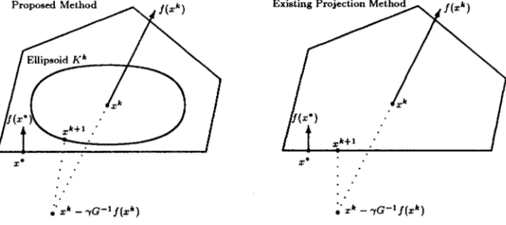
1 from the proof of Proposition 1, we get x"+! E int(K)

Figure 1 is a schematic representation of the proposed scheme. Unlike the existing projection methods whose generic iteration solves VIe K, Jk) (equivalently projecting xk

-'YG-1 J(x k) onto any convex set K with respect to G-norm), the proposed method solves

VI(Kk, Jk).

4. Convergence property

It is known that iterative projection methods (see Dafermos [5], and Pang and Chan [10)) monotonically converges to a solution x*, if the relaxation parameter 'Y is chosen sufficiently small [5] under the assumptions that

f

is continuously differentiable and strictly monotone and that K is compact. This convergence discussion is rather theoretical, since a small 'Y results in slow convergence often making it unacceptable as a realistic solution scheme. Our suggestion is to replace K with an ellipsoid K" for projection operation. Now the question is whether Dafermos' style of convergence, even if theoretical, is maintained under the ellipsoidal approximation. It is affirmative. That is, choosing 'Y sufficiently small, it can be shown to converge to a solution as well under the assumptions that

f

Figure 1: Schematic representation of V I(Kk, fk)

is continuously differentiable and "il f( x) is positive definte on K and that the problem has a bounded solution. To prove the convergence, some lemmas and propositions are presented.

Lemma 1 If xk - ,G-1 _{f(x k)}

_rt

_{int(J(), then there exi3t3 6}

_>

_{0 3uch that}

Proof: Since the ellipsoid

is contained in K,

Hence,

1

If a denotes

,QZ

G-l

f(x k), it could be expressed as

On the other hand, rewriting (10),

Xk+l - xk

=

-,(G

+

{ikQd-1f(x k), (G

+

{ikQk)(X k+1 - xk)

=

-,f(x k), ,f(xk)

+

G(Xk+l - Xk)

=

-{ikQk(Xk+l _ xk),

Letting a and M denote Vf(xk)TQ;;l f(x k ) and Q~!G(G + iLkQk)-lQk(G + iLkQk)-lGQ~!

respectively for notational simplicity, we get

(f(xk)

+

,

.!.G(Xk+l _ xkjf(xk _ Xk+l)

=

_a(xk+1 _ xkfQk(:rk __ x k+1)

=

a,f(xkf(G

+

JikQk)-1Qk(G

+

JikQk)-1 f(xkh.

= aaT M

a

~

mnllal12

>

am,

where in is the minimum eigenvalue of the positive definite matrix M . •

Lemma 2 There exists

'?t

>

0 such that

(f(xk)

+

.!.G(xk+1 - xk)f(x" - Xk+l)

,

~

0,

for any , ~

'11

where x* is a solution to V I(/(, I).

Proof:

case 1: when xk

_,G-

1 _f(xk

) E int(K)

Xk+l _ xk = _~yG-1 f(x k).

f(x k)

+

.!.G(xk+1 - xk)

,

=

o.

case 2: when xk -,G-1 f(x k)

f/.

int(/{) From Lemma 1 and (10),

(f(xk)

+

.!.G(xk+1 - xk)f(x" _ Xk+1'1

,

,

(f(xk)

+

.!.G(xk+1 - xk)f(xk - Xk+1')

,

. ,

+

(f(xk)

+

.!.G(xk+1 _ xk))T(x" _ xk)

>

6

+

[J( a;k) - G( G

+

JikQk )-1 f( xk)f (.x" - xk)

= 6

+

f(x kf[l - G(G

+

l'aQk)-l]T(x" - xk) ~ 0,

for sufficiently small" since 1-G(G

+

,aQkj-1 converges to 0

as,

approaches

o . •

Lemma 3 If x" and Xk are bounded, then there exists

'12

>

0 such that

for any , ~

'12

and t E [0,1] where x" is a solution to V I(K, I).

Proof: Let

x

be a point that maximizes the left hand side of the above inequality over the convex combination of xk and x". Then

111

-,G-!Vf(tx*

+

(1-t)xk)G-~'1I2

<

111 -

/'G-tvf(x)G- tIl2

= sup yT(I

-,G-tv

f(x)G-!f(I -- /,G-tv f(x)G-!)y

IIYiI=l

<

1 - 2/, inf yTG-tv f(x)G-!y

+

1,2 sup yTG-!V f(xfG- 1V f(x)G-t y

IIYII=1 lIylI=1

for'Y

<

2in/ L, where in and L are minimum and maximum eigenvalues of the symmetric parts of C-~Vf(x)C-~ and C-~Vf(xfC-IVf(x)C-~ respectively. Note that Vf(x) is positive definite and bounded . •

Proposition 2 Suppose that xk and x* are bounded. If'Y is sufficiently small (i.e., 'Y :::; min{"h,7'2}), then

where x* is a solution to V I(K, I).

Proof: As Xk+l E K and x* solves VI(K, I)

(11)

From Lemma 2 (12)

Adding (11) and (12), we get

Then

(f(x*) - f(x k)

+

!C(xk - x*)f(Xk+l - x*) - !llxk+1 - x*lI&

~

o.

'Y 'Y

[f(x*) - f(x k)

+

!C(xk - x*)]TC-!C!(xk+1 - x*)

'Y

<

IIC-~(f(x*)

- f(x k))

+

!C!(xk - x*)lIlIxk+1 - x*IIG. 'Y

Dividing by IIXk+1 - x*IIG, we get

IIXk+1 - x*IIG :::; 'Yllc-t(f(x*) - f(x k))

+

!C~(xk

- x*)II.

'Y By the mean value theorem, there exists t

E [0,1]

such that

'YIIC-i(f(x*) - f(x k))

+

!Ci(xk - x*)1I

'Y

=

'YIIC-!Vf(tx*

+

(1-t)Xk)(X* - xk)

+

!C!(xk - x*)11

'Y

=

II{ -'YC-~V f(tx*

+

(1 - t}xk)

+

C~}(xk - x*)1I

=

11{ -'YC-iv f(tx*

+

(1 - t)xk)C-t

+

I)}Ct(xk - x*)1I

<

II-'YC-!Vf(tx* +(l-t)xk)C-! +IIIII(xk -x*)IIG Combining this with the result of Lemma 3, we finally get

By applying mathematical induction to Proposition 2, we know that the sequence {xk}

is bounded, since x* and Xl are bounded. Hence, we finally conclude that the sequence

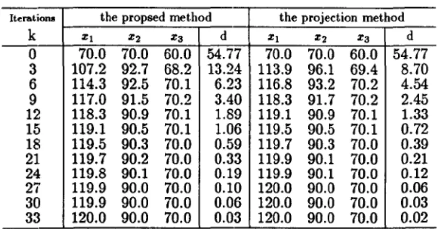
Table 1: Computational Results of Example 1

Iterations the propsed method the projection method

k Z1 Z2 Z3 d Z1 Z2 Z3 d 0 70.0 70.0 60.0 54.77 70.0 70.0 60.0 54.77 3 107.2 92.7 68.2 13.24 113.9 96.1 69.4 8.70 6 114.3 92.5 70.1 6.23 116.8 93.2 70.2 4.54 9 117.0 91.5 70.2 3.40 118.3 91.7 70.2 2.45 12 118.3 90.9 70.1 1.89 119.1 90.9 70.1 1.33 15 119.1 90.5 70.1 1.06 119.5 90.5 70.1 0.72 18 119.5 90.3 70.0 0.59 119.7 90.3 70.0 0.39 21 119.7 90.2 70.0 0.33 119.9 90.1 70.0 0.21 24 119.8 90.1 70.0 0.19 119.9 90.1 70.0 0.12 27 119.9 90.0 70.0 0.10 120.0 90.0 70.0 0.06 30 119.9 90.0 70.0 0.06 120.0 90.0 70.0 0.03 33 120.0 90.0 70.0 0.03 120.0 90.0 70.0 0.02

d: the Euclidean distance from the solution

5. Numerical results

Small-sized traffic equilibrium problems are solved by both the proposed algorithm and a standard projection method to compare computational performances. The result is promising in the sense that our method requires only a few additional iterations compared to the projection method to get the equal accuracy, even though our method involves more approximation at each iteration. The program was coded in Turbo-basic and run on a IBM 486DX2 PC.

The first exanlple (Example 1) is taken from [4]. To fit into our standard form, the equalities representing set K are converted into inequalities and function

f

is transformed into a suitable form. The function

f

is given by

f(x) =

(~~2 ;~ -~)

x - (

~~~~

) ,

-1 45 3300

and the set K is given by

K

=

{x

I

Xl

+

X2 ~ 210,x3 ~ 120,xj ~ 0 Vi}.

The solution of this problem is known to be (120,90,70). The matrix G is chosen as the diagonal matrix whose elements are equal to the diagonal elements of the linear part of

f.

i.e.,

G =

(3~ 3~ ~),

o

0 45

and the value of'Y is set to 0.5. Computaional results with the starting point (70,70,60) are summarized in Table 1.

The column named "d" represents the Euclidean distance of each iterate from the known solution. This shows that our method needs about three more iterations than the projection method to get the equivalent accuracy. Similar computational results are shown in Table 2 for other examples, where 4 to 6 more iterations are required. Examples in Table 2 are of the same type as Example 1, i.e., they are traffic equilibrium problems. As far as

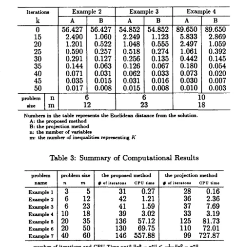
Table 2: Computational results of other examples

Iterations Example 2 Example 3 Example 4

k A B A B A 0 56.427 56.427 54.852 54.852 89.650 15 2.490 1.060 2.249 1.123 5.833 20 1.201 0.522 1.048 0.555 2.497 25 0.590 0.257 0.518 0.274 1.061 30 0.291 0.127 0.256 0.135 0.442 35 0.144 0.063 0.126 0.067 0.180 40 0.071 0.031 0.062 0.033 0.073 45 0.035 0.015 0.031 0.016 0.030 50 0.017 0.008 0.015 0.008 0.010 problem

l

n 6 6 size m 12 23

Numbers in the table represents the Euclidean distance from the solution. A: the proposed method

B: the projection method n: the number of variables

m: the number of inequalities representing K

B 89.650 2.869 1.059 0.392 0.145 0.054 0.020 0.007 0.003 10 18

Table 3: Summary of Computational Results

problem problem size the proposed method the projection method name n m .. of iter.lou CPU time "# of i'eraton • CPU lime

Example 1 3 5 31 0.27 28 0.16 Example 2 6 12 42 1.21 36 2.36 Example 3 ₆ 23 _{41 1.59} 37 _7.69 Example 4 10 18 ₃₉ 3.02 33 3.19 Example 5 20 35 136 57.12 125 81.73 Example 6 20 50 130 69.75 110 72.01 Example 7 40 60 146 557.88 99 727.87

number of iterations and CPU Time until lI"k - ,,°11 ~

tfoo

11,,0 - ,,°11

the number of iterations required is concerned, our method is only a little bit late despite the approximation applied to the set K. Table 3 summarizes the computational results of our limited computational experience. Similar results in terms of required number of iterations are shown for Example 4, Example 5 and Example 6 which was randomly generated. Note that we do not mention the total CPU time due to the subjectivity in selecting a QP algorithm for the existing projection method.

In any event, this relatively slow convergence (in terms of required iterations) could be compensated by time saving from the closed-form solution of each iteration. Especially when the set K is not so simple, e.g., many inequalities representing K, a substantial computational burden may be incurred for each iteration of the projection method. On the contrary, computational burden of our method in this case is surmountable, since the size of the matrix to be inverted depends only on the number of variables.

6. A practical version

We presented an ellipsoidal projection method whose generic iterations are carried out in a closed-form. Because we are attempting to approximate a polyhedral set by an inscribed ellipsoid, it would be desirable to choose the radius of the ellipsoid as close as possible to 1.

However, there is no theoretical guarantee that the radius of the ellipsoid does not become too small. To avoid such a pitfall, we suggest a practical version with an additional step that gives safety against the possible risk of small radius.

Unlike the original version where xk+l = xk -/(G+iikQk)-l f(x k), the practical version determines Xk+l somewhere on the line segment between xk -/(G

+

iikQk)-lf(xk) and xk -IG-1f(xk) with the restriction Xk+l E K. The additional step can be carried out without much computation, since it is only a standard minimum ratio test. The practical version can be summarized as follows:

(13)

qk

=

xk -IG-1 f(x k)

If qk E int( K) then xk+1 = qk

else ilk = I/i-f(-x-k)-T-Q-;-lf-(-x-k) yk = xk '-/(G

+

iikQktlf(xk) dk = qk __ yk

t

= max{ t

>

0

I

yk

+

tdk E K} f3

=

lot

xk+1 = yk

+

f3dk.

where 0

<

10

<

1 is a given constant. Note that 0

<

f3 ~ 10

<

1, since

t

~ 1.

Now, we will briefly show that the theoretical convergence is maintained under the pratical version. When xk -IG-l f( xk) E int( K), the convergence property of the practical version is the same as the original version since no additional step is performed in the practical version. In the remainder of this section, we will discuss the convergence property of the practical version when xk - IG-l f( xk)

rt

int( K).

Noting that Xk+l in the previous sections is denoted by yk in this section, the conclusion of Lemma 1 can be rewritten as follows:

There exists 6

>

0 such that (14)

Next, we will show that the conclusion of Lemma 2 is valid under the practical version when xk -IG-1 _{f(x k)}

rt

_{int(K). We get from (13)}

Xk+1 _ xk = yk

+

f3dk _ :rk = yk

+

f3 qk _ f3 yk _ xk

= (1 - (3)yk

+

f3xk -1f3G-1 _{f(x k) - xk}

= (1 - (3)(yk - Xk) - "If3G-1 _{f(x k).} Hence, it is enou!~h to show that there exists ~il

>

0 such that

(f(Xk)

+

.!.G(xk+1 - xk)f(x· _ x k+1) "I

= (1 - (3)(f(x k)

+

.!.G(l-- xk»T(x· - yk - f3dk)

~

0,

"I

(f(Xk)

+

.!.G(yk _ xk)f(xk _ yk)

+

(f(Xk)

+

.!.G(yk - xk)f(x* - xk --(3dk)

~ ~

>

b

+

[f(x k) - G(G

+

PkQkflf(xk)f(x* - xk - (3dk)

b

+

f(xk)T[I - G(G

+

~aQkrlf(x* - xk - (3dk) ~ 0,

for sufficiently small~. With this result, it is evident that Lemma 3 and Proposition 2 are valid and that the sequence generated by the practical version also converges to the solution x*.

Acknowledgment: The authors acknowledge the valuable comments and suggestions from Professor Fukushima. The practical version of section 6 is heavily due to his sugges-tions.

References

[1] Ahn, B., Computation of market equilibria for policy analysis: the project independent evaluation system (PIES) approach, Gurland, New York (1979).

[2] Barnes, E.R, "A variation on Karmarkar's algorithm for solving linear programming problems", Mathematical Programming, Vol. 36 (1986) 174-182.

[3] Bertsekas, D.P. and Gafni, E.M., "Projection methods for variational inequalities with application to the traffic assignment problem", Mathematical Programming Study, Vol. 17 (1982) 139-159.

[4] Dafermos, S., "'Traffic equilibrium and variational inequalities", Transportation Sci-ence, Vol. 14 (1980) 42-54.

[5] Dafermos, S., "An iterative scheme for variational inequalities", Mathematical Pro-gramming, Vol. 26 (1983) 40-47.

[6] Friesz, T.L., Harker P.T. and Tobin, RL., "Alternative algorithms for the general network spatial price equilibrium problem", Journal of Regional Science, Vol. 24 (1984) 473-503.

[7] Fukushima, M., "A relaxed projection method for variational inequalities", Mathe-matical Programming, Vol. 35 (1986) 58-70.

[8] Gabay, D. and Moulin, H., "On the uniqueness and stability of Nash-equilibria in noncooperative games", in: A. Bensoussan, P. Kleindorferand C.S. Tapiero, eds., Applied Stochastic Control in Economatrics and Management Science, North Hol-land, Amsterdam (1980) 271-292.

[9] Harker, P.T. and Pang, J.S., "Finite-dimensional variational inequality and nonlinear complementarity problems: a survey of theory, algorithms and applications", Math-ematical Programming, Vol. 48 (1990) 161-220.

[10] Pang J.S. and Chan, D., "Iterative methods for variational and complementary prob-lems", Mathematical Programming, Vol. 24 (1982) 284-313.

Seung-gyu BAEK: Faculty of Department of Business Administration Soonchunhyang University 53-1 Shinchang-myon, Asan Chung-nam 337-745, Korea