Utilizing an invariance of Krylov subspaces with the Jacobi-Davidson method for eigenvalue problems (Fusion of theory and practice in applied mathematics and computational science)
6
0
0
全文
(2) 66. derive. version of the JD method. To show the convergence behavior methods, we report some numerical experiments in §4. Finally, we. a new. of the. summarize the. report in §5.. Throughout the paper, the n\times n identity matrix is denoted by I The transpose and conjugate transpose are denoted by the superscripts (\cdot)^{\mathrm{T} and (\cdot)^{*} respectively. The m dimensional Krylov subspace with respect to A and a vector v, \mathrm{s}\mathrm{p}\mathrm{a}\mathrm{n}\{v, Av, . . . , A^{m-1}v\} is denoted by \mathcal{K}_{m}(A, v) The 2‐norm is denoted by \Vert \Vert For subspaces S_{1} and S_{2} the direct sum of S_{1} and S_{2}, \mathrm{s}\mathrm{p}\mathrm{a}\mathrm{n}\{s_{1}+s_{2}|s_{i}\in S_{i}, i=1, 2\} is denoted by S_{1}\oplus S_{2} In the case of S_{1}\perp S_{2}, S_{1}\oplus S_{2} is especially denoted by S_{1}S_{2} The complementary projector of v for \Vert v\Vert=1 is defined by I-vv^{*} and is denoted by P_{\perp v}. .. ,. ,. .. .. ,. .. ,. .. 2. The JD method. Suppose a subspace \mathcal{Q}_{k} is generated at the kth iteration in the JD method, and an approximation ($\theta$^{(k)}, u^{(k)}) of a wanted eigenpair ( $\lambda$, x) is produced by using \mathcal{Q}_{k} Here, \Vert u^{(k)}\Vert=1 and $\theta$^{(k)} :=(u^{(k)})^{*}Au^{(k)} The residual vector is defined by r^{(k)} :=Au^{(k)}-$\theta$^{(k)}u^{(k)} If the residual norm \Vert r^{(k)}\Vert is enough .. .. .. small,. the iteration is. stopped. Otherwise, the subspace will be expanded for a better approximated eigenpair. Here, we describe how to generate a next basis vector to expand the subspace.. [6]. The JD method. is based. on. [4]. the Jacobis idea. that is to find. a. :=x-u^{(k)} satisfying the orthogonality t\perp u^{(k)} Since the eigenvector x will be found in a subspace \mathcal{Q}_{k}\oplus \mathrm{s}\mathrm{p}\mathrm{a}\mathrm{n}\{t\} the JD method searches for the correction vector t to expand the subspace \mathcal{Q}_{k} By (1), t correction vector t. .. ,. .. satisfies. A(u^{(k)}+t)= $\lambda$(u^{(k)}+t). (2). .. (A- $\lambda$ I)t=-r^{(k)}+( $\lambda-\theta$^{(k)})u^{(k)} Multiplying the both sides in this equation by P_{\perp u^{(k)}} results in P_{\perp u^{(k)}}(A- $\lambda$ I)t=-r^{(k)} Since From. (2),. it follows that. .. .. t\perp u^{(k)}. ,. we. have. P_{\perp u^{(k)}}(A- $\lambda$ I)P_{\perp u^{(k)}}t=-r^{(k)} If the unknown. keeping. the. eigenvalue orthogonality. (3). .. (3) is replaced by its approximation $\theta$^{(k)} while u^{(k)} then we reach a correction equation [6]:. $\lambda$ in to. ,. ,. P_{\perp u^{(k)}}(A-$\theta$^{(k)}I)P_{\perp u^{(k)}}t_{\mathrm{J}\mathrm{D}}=-r^{(k)} where. t_{\mathrm{J}\mathrm{D} \perp u^{(k)}. If. $\theta$^{(k)}. ,. (4). good approximation of $\lambda$ an approximate cor‐ produced by solving the linear equation (4). To compute the correction vector, it was proposed in [6] that (4) is ap‐ proximately solved by an iterative method, e.g., a few steps of GMRES [5]. .. rection vector will be. is. a. ,.
(3) 67. Finally, an approximate solution of (4) is orthonormalized against the basis of \mathcal{Q}_{k} and then the resulting vector is the next basis vector to expand \mathcal{Q}_{k}. ,. 3. New. We show vector. v. approach a. to the correction vector. of. decomposition. with. \Vert v\Vert=1. for any. Krylov subspace $\gamma$\in \mathbb{C} :. a. with respect to A and. \mathcal{K}_{m}(A, v)=\mathrm{s}\mathrm{p}\mathrm{a}\mathrm{n}\{v\}\mathcal{K}_{m-1}(P_{\perp v}(A- $\gamma$ I)P_{\perp v}, P_{\perp v}Av) We will utilize. (5). to. compute the correction. expansion of the subspace \mathcal{Q}_{k}. As supposed in §2, the approximate. vector. (5). .. approximately. a. for alter‐. native. the. subspace \mathcal{Q}_{k} equation. where. t_{\star}\perp u^{(k)}. .. eigenpair. For the correction vector,. ($\theta$^{(k)}, u^{(k)}). we. consider. P_{\perp u^{(k)}}(A-$\gamma$^{(k)}I)P_{\perp u^{(k)}}t_{\star}=-r^{(k)}. and. $\gamma$^{(k)}\in \mathbb{C}. is undetermined.. As. given by using solving a linear. is. (6). ,. we. have reviewed the. §2, appropriate setting $\gamma$^{(k)} to a well (6) approximated eigenvalue. To this end, let us utilize (5) for $\gamma$=$\gamma$^{(k)} and v= u^{(k)} ; hence, P_{\perp v}Av=r^{(k)} If we generate a Krylov subspace \mathcal{K}_{m}(A, u^{(k)}) then we also have a Krylov subspace \mathcal{K}_{m-1}(P_{\perp u^{(k)}}(A-$\gamma$^{(k)}I)P_{\perp u^{(k)}}, r^{(k)}) The \mathcal{K}_{m}(A, u^{(k)}) can be used to compute an approximate eigenvalue for $\gamma$^{(k)} while \mathcal{K}_{m-1}(P_{\perp u^{(k)}}(A-$\gamma$^{(k)}I)P_{\perp u^{(k)}}, r^{(k)}) can be used to compute an approximate solution t_{\star}^{(k)} of the linear equation (6) (initial guess is supposed to be 0 ). From this observation, we consider an approach to the correction vector: we generate the Krylov subspace \mathcal{K}_{m}(A, u^{(k)}) ; JD method in. to solve. it is. after. .. ,. .. ,. not. the. only to compute Krylov subspace. an. \mathcal{K}_{m}(A, u^{(k)}). In this way,. $\gamma$^{(k)}. in. approximate solution. an. (6) by using. ;. t_{\star}^{(k)} of (6) \mathcal{K}_{m-1}(P_{\perp u^{(k)}}(A-$\gamma$^{(k)}I)P_{\perp u^{(k)}}, r^{(k)}). but also to compute. Krylov subspace. approximate eigenvalue for. by using. the. .. the two. Krylov subspaces for the correction vector by generating only one Krylov subspace. Finally, an approximate solution of (6) is orthonormalized against the basis of \mathcal{Q}_{k} and then the resulting vector is the next basis vector to expand \mathcal{Q}_{k}. we can use. ,. 4. Numerical. Computational run. experiments. environment is MATLAB. (version 7.10.0.499 (\mathrm{R}2010\mathrm{a})64\mathrm{b}\mathrm{i}\mathrm{t} ) (3.1 GHz). In all experiments, an. under Linux with Intel Core i7‐3770S. initial vector is. u^{(1)}=[1. ,. .. .. .. ,. 1. ]^{\mathrm{T} /\sqrt{n}. ,. and iterations stop if. \Vert r^{(k)}\Vert\leq 10^{-10}.
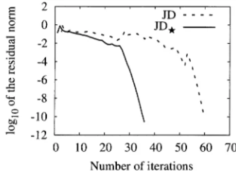
(4) 68. We consider the. of which the. eigenvalue problem of an. real. n\times n. nonsymmetric. A=\left{\begin{ar y}{l a_{1}&a_{3}& 0a_{3}\ a_{2}0&a_{1}&a_{3}&a_{2}&a_{1} \end{ar y}\ight},. eigenvalues. are. $\lambda$_{\mathcal{J} =a_{1}+2\displaystyle \sqrt{a_{2}a_{3} \cos\frac{\dot{j} $\pi$}{n+1} (j=1, \ldots, n) The. following. methods. JD:. The JD method. \mathrm{J}\mathrm{D}_{\star} :. The. new. are. .. compared. 10 steps of GMRES.. using. version of the JD method with m=11.. Note that these methods a. require 10 matrix‐vector multiplications to generate problems are determined as follows.. basis vector per iteration. The. (a). The target is the and a_{3}=1.6.. (b). The target is the eigenvalue closest to -2.1+0 li for n=100, a_{2}=1.0 , and a_{3}=0.9 , which is the interior eigenvalue $\lambda$_{52}.. largest eigenvalue $\lambda$_{n}. for. n=100, a_{1}=-2.0, a_{2}=1.0,. .. We show the convergence From Fig. 1, we observe that both. 5. matrix. cases. (a). and. Concluding. history of the residual norm \Vert r^{(k)}\Vert \mathrm{J}\mathrm{D}_{\star} converges slightly faster than. a_{1}=-2.0, in. Fig.. 1.. JD in the. (b).. remarks. To generate a subspace, equation which is known. have focused. approximate solving a linear as a correction equation. The equation is deter‐ mined by an approximation of a wanted eigenvalue, and a good approxima‐ tion is appropriate to find the eigenvector which corresponds to the wanted eigenvalue in the subspace. In this report, we have considered utilizing an invariance of Krylov sub‐ spaces to use one Krylov subspace for two aims. The first aim is to generate approximate eigenvalues that determine correction equations. The second aim is to solve the equations approximately. By the choice of a correction equation and its approximate solution, we have proposed a new version of the we. on.
(5) 69. \dot{unerli\math{o}$Xi. \displaytemhr{E}\fac$Ximthr{o}. \overlin{cfa\mthr{o}inyafkc9=. \overlin{mathrB}^{$\Xi sgma$3}. \mathrm{q}\overline{\cir }. 4\dot{\circ}. \overline{\infty}. \underline{$\omega$}. \underli {\mathr{n}^$\omega$}. \underlin{=$\omega$}. \underli{matho}\ rm{^\facmthr{o}\am}. \underli{matho}\ rm{^\facmthr{o}\am} 0. 10. 20. 30405060. 0 10 203040506070. Number of iterations. (a) Computing. the exterior. Figure. Number of iterations. 1: The convergence. Jacobi‐Davidson method. In the value. (b) Computing. eigenvalue.. history. new. the interior. of the residual. method,. a. better. eigenvalue.. norm.. approximated eigen‐. be put into the correction equation, while keeping the number of matrix‐vector multiplications per iteration the same as the Jacobi‐Davidson can. method.. Numerical. experiments show that the new method has attrac‐ behavior in comparison with the Jacobi‐Davidson method.. tive convergence Therefore, we conclude that the is. promising for computing. new. few. a. version of the Jacobi‐Davidson method. eigenpairs of. a. large. sparse matrix.. Acknowledgment This work. was. partially supported by KAKENHI Grant. number 24760061.. References. [1]. BAI, J. DEMMEL, J. DONGARRA, A. RUHE, AND H. VAN DER VORST, Templates for the Solution of Algebraic Eigenvalue Problems: A Practical Guide, SIAM, Philadelphia, 2000.. [2]. FOKKEMA, G. L. G. SLEIJPEN, AND H. A. VAN DER VORST, Jacobi‐Davidson style QR and QZ algorithms for the reduction of matrix pencils, SIAM J. Sci. Comput., 20 (1998), pp. 94‐125.. [3]. M. E. HOCHSTENBACH. Z.. D. R.. GAMM‐Mitt.,. 29. AND. (2006),. Y.. NOTAY,. pp. 368‐382.. The Jacobi‐Davidson. method,.
(6) 70. [4]. JACOBI, Ueber ein leichtes Verfahren, die in der Theorie der Säcularstörungen vorkommenden Gleichungen numerisch aufzulösen, J. Reine Angew. Math., (1846), pp. 51‐94.. [5]. Y. SAAD. [6]. G. L. G. SLEIJPEN. AND. iteration method. linear. C. G. J.. SCHULTZ, GMRES: A generalized minimal resid‐ ual algorithm for solving nonsymmetric linear systems, SIAM J. Sci. Stat. Comput., 7 (1986), pp. 856‐869. AND. M. H.. \partial. Appl.,. 17. (1996),. for. H. A. VAN. VORST, A Jacobi‐Davidson eigenvalue problems, SIAM J. Matrix Anal.. pp. 401‐425.. DER.
(7)
図
関連したドキュメント
This paper derives a priori error estimates for a special finite element discretization based on component mode synthesis.. The a priori error bounds state the explicit dependency
The strategy to prove Proposition 3.4 is to apply Lemma 3.5 to the subspace X := (A p,2 ·v 0 ) ⊥ which is the orthogonal for the invariant form h·, ·i p,g of the cyclic space
A generalization of Theorem 12.4.1 in [20] to the generalized eigenvalue problem for (A, M ) provides an upper bound for the approximation error of the smallest Ritz value in K k (x
Kilbas; Conditions of the existence of a classical solution of a Cauchy type problem for the diffusion equation with the Riemann-Liouville partial derivative, Differential Equations,
The last sections present two simple applications showing how the EB property may be used in the contexts where it holds: in Section 7 we give an alternative proof of
Applications of msets in Logic Programming languages is found to over- come “computational inefficiency” inherent in otherwise situation, especially in solving a sweep of
Shi, “The essential norm of a composition operator on the Bloch space in polydiscs,” Chinese Journal of Contemporary Mathematics, vol. Chen, “Weighted composition operators from Fp,
We provide an efficient formula for the colored Jones function of the simplest hyperbolic non-2-bridge knot, and using this formula, we provide numerical evidence for the
