Master’s Thesis
A Regularized Outer Approximation Method for Monotone Semi-Infinite Variational Inequality Problems
Guidance
Professor Masao FUKUSHIMA
Masaki KONO
Department of Applied Mathematics and Physics Graduate School of Informatics
Kyoto University
KYOTO UNIVER SIT
Y F
OU
ND E D 1897 KYOTO JAPAN
February 2013
Abstract
We study the variational inequality problem (VIP) whose feasible set is defined by
infinitely many convex inequalities. It is called the semi-infinite variational inequality
problem (SIVIP). For solving SIVIP, we propose an algorithm combining an outer
approximation method with a regularization method, which solves a VIP with a finite
number of inequality constraints approximately at each iteration. It makes use of
the regularized gap function to specify a criterion for approximate solutions of such
VIPs. We establish global convergence of the proposed algorithm by assuming the
monotonicity of the problem, Slater’s condition, and the existence of a solution. We
report some numerical results to examine the efficacy of the algorithm.
Contents
1 Introduction 1
2 Preliminaries 2
3 Algorithm for the strongly monotone SIVIP 3
4 Algorithm for the monotone SIVIP 7
5 Numerical experiments 10
6 Conclusion 13
1 Introduction
The variational inequality problem (VIP), denoted by VI(S, F ), is to find a point x
∗∈ R n such that
x
∗∈ S, ⟨ F (x
∗), x − x
∗⟩ ≥ 0 for all x ∈ S,
where S is a nonempty closed convex subset of R n , F is a mapping from R n into itself, and
⟨· , ·⟩ denotes the inner product in R n . Throughout the paper, we assume that the mapping F is continuously differentiable. The VIP has been used to study various equilibrium models in economics, operations research, transportation and regional science. A survey of the theory, algorithms and applications of the VIP can be found in [8, 13]. The VIP has been well studied and a lot of algorithms are available for solving it. However, many of the existing algorithms work practically only when S exhibits a certain tractable structure such as the nonnegative orthant of R n or a polyhedral set.
In this paper, we consider VI(S, F ) with S particularly defined by
S = { x ∈ R n | g (x, t) ≤ 0 for all t ∈ T } , (1.1) where T ⊂ R m is a nonempty compact set with infinitely many elements and g : R n × T → R is a continuous function such that g( · , t) is a convex function for each fixed t ∈ T . Since there are infinitely many constraints, the VIP with S defined by (1.1) is called the semi-infinite variational inequality problem (SIVIP). In the remainder of this parer, we let SIVI(S, F ) denote this problem. Note that S can be expressed as
S = { x ∈ R n | h(x) ≤ 0 } , (1.2)
where the function h : R n → R is defined by h(x) = max
t
∈T g(x, t). (1.3)
Despite numerous works on the VIP and the semi-infinite programming problem (SIP) [19, 22], which is the mathematical programming problem with the feasible set defined by (1.1), the study on the theory and algorithms for solving the SIVIP is relatively recent.
Since S is defined by infinitely many inequalities, it is hard to deal with the problem directly in practice. Then, for solving VI(S, F ) with such S, several algorithms have been proposed on the basis of an outer approximation method. The fundamental idea underlying the outer approximation method is to generate a sequence { x k } by solving subproblems whose feasible sets S k contain S and are relatively easy to deal with. Fukushima [11] intro- duced a relaxed projection method for solving VI(S, F ) where S is defined by (1.2) with a general convex function h. This method computes at each iteration the projection onto a half space S k defined by using the subdifferential of h at the current iterate x k . It has been showed that this method is globally convergent under the strong monotonicity assumption on F . A method with S k replaced by a general half space separating x k from S has been proposed by Censor and Gibali [7]. Bello Cruz and Iusem [2] provided an algorithm based on the method in [11] and showed its global convergence under the weaker condition that F is paramonotone [15]. Moreover, the same authors [3] presented a relaxed projection-type method which is globally convergent under the mere monotonicity assumption on F .
For SIVI(S, F ) with S particularly defined by (1.1), there have been proposed several
methods on the basis of the outer approximation method. These methods solve VI(S k , F )
at each iteration k, where S k is an outer approximation of S defined by finitely many inequalities. Under the assumption that F is paramonotone and S is compact, Burachik et al.
[4] proposed an outer approximation scheme for solving the SIVIP. Assuming S is compact and F is Lipschitz continuous and pseudomonotone-plus [17], implementable algorithms have been presented in [9, 21]. Under the same assumptions, Fang et al. [10] provided an inexact method which uses an approximate solution of VI(S k , F ) at each iteration. They use the gap function value as a criterion for an approximate solution, where the gap function is a merit function for the VIP proposed by Auslender [1]. Without the compactness of S, Burachik et al. [6] introduced a scheme combining the outer approximation method with a regularization method, which solves VI(S k , F k ) at each iteration, where F k is an approximate mapping of F . They proved that when F is paramonotone, a sequence of exact solutions of VI(S k , F k ) is bounded and any of its accumulation points solves SIVI(S, F ).
We propose an algorithm for solving the SIVIP, which is an implementable version of the regularized outer approximation scheme [6]. This method needs only an approximate solution of VI(S k , F k ), while the scheme in [6] assumes the exact solution of VI(S k , F k ).
We use the regularized gap function [12] to specify a criterion for approximate solution of VI(S k , F k ). Moreover, we establish global convergence of the proposed algorithm by assuming the existence of a solution of SIVI(S, F ), Slater’s condition, and the monotonicity of F , which is a weaker assumption on F than the paramonotonicity assumed in [6].
This paper is organized as follows. In Section 2, we review some preliminary results concerning monotone mappings and the regularized gap function. In Section 3, we propose an outer approximation method and show that it has global convergence under the strong monotonicity assumption on the mapping F . In Section 4, we provide an algorithm combin- ing the method proposed in Section 3 with a regularization method, and establish its global convergence under the mere monotonicity assumption on the mapping F . In Section 5, we give some numerical results to examine the efficacy of the proposed algorithm. In Section 6, we conclude the paper with some remarks.
2 Preliminaries
In this section, we simply assume that S is a general nonempty closed convex set. For VI(S, F ), Auslender [1] showed that the gap function f
0: R n → R ∪ { + ∞ } defined by
f
0(x) = sup
y
∈S ⟨ F (x), x − y ⟩
attains its minimum on S at a solution of VI(S, F ). However, the function f
0is in general nondifferentiable and may even fail to be finite-valued. To overcome such drawbacks of the gap function, Fukushima [12] proposed the regularized gap function f α : R n → R defined by
f α (x) = sup
y
∈S
{
⟨ F (x), x − y ⟩ − 1
2 α ∥ y − x ∥
2}
,
where α > 0 is a parameter. This function enjoys a similar property to that of the gap function, as shown in the following proposition.
Proposition 2.1. [12, Theorem 3.1] The function f α satisfies f α (x) ≥ 0 for all x ∈ S.
Moreover, f α (x) = 0 and x ∈ S if and only if x solves VI(S, F ). Hence x solves VI(S, F ) if
and only if it solves the following optimization problem and f α (x) = 0:
minimize f α (x) subject to x ∈ S.
Unlike the gap function f
0, the regularized gap function f α is always finite-valued. When the mapping F is continuously differentiable, so is f α . In addition, the function f α has some useful properties. Several methods utilizing this function have been proposed for solving VI(S, F) [24, 25, 26].
Recall that the mapping F : R n → R n is said to be monotone if
⟨ F (x) − F (y), x − y ⟩ ≥ 0 for any x, y ∈ R n , (2.1) strictly monotone on S if strict inequality holds in (2.1) whenever x ̸ = y, and strongly monotone with modulus µ > 0 if
⟨ F (x) − F (y), x − y ⟩ ≥ µ ∥ x − y ∥
2for any x, y ∈ R n .
Clearly any strongly monotone mapping is strictly monotone, and any strictly monotone mapping is monotone.
3 Algorithm for the strongly monotone SIVIP
In this section, we make the following assumption, which ensures that SIVI(S, F ) has the unique solution x
∗.
Assumption 3.1. The mapping F : R n → R n is strongly monotone with modulus µ > 0.
We propose a method for solving SIVI(S, F ) with S given by (1.1) and show its global convergence under Assumption 3.1. The proposed algorithm consists of major iterations and inner iterations within each major iteration. On the rth inner iteration of the kth major iteration, a nonempty finite set T k,r ⊂ T is given. We define the set S k,r ⊆ R n by
S k,r = { x ∈ R n | g (x, t) ≤ 0 for all t ∈ T k,r } , (3.1) and consider VI(S k,r , F ), which is easier than SIVI(S, F ) to deal with, since S k,r consists of finitely many constraints. Moreover, define the function f α k,r : R n → R by
f α k,r (x) = sup
y
∈S
k,r{
⟨ F (x), x − y ⟩ − 1
2 α ∥ y − x ∥
2}
, (3.2)
where α > 0. Note that the maximum on the right-hand side of (3.2) is always attained at some point y = y α k,r (x) uniquely, that is, y α k,r (x) is the unique solution y to the quadratic programming problem
QP k,r α (x) : minimize
y
∈Rn1
2
α ∥ y − x ∥
2+ ⟨ F (x), y − x ⟩ subject to g(y, t) ≤ 0 for all t ∈ T k,r . Thus, the function f α k,r can be written as
f α k,r (x) = ⟨
F (x), x − y α k,r (x) ⟩
− 1
2 α y α k,r (x) − x
2.
The function f α k,r is the regularized gap function for VI(S k,r , F ), which is continuously dif-
ferentiable.
Proposition 3.2. [12, Theorem 3.2] The function f α k,r is continuously differentiable and its gradient is given by
∇ f α k,r (x) = F (x) − [ ∇ F (x) − αI](y α k,r (x) − x), where ∇ F (x) is the Jacobian matrix and I ∈ R n
×n is the identity matrix.
By Proposition 2.1, VI(S k,r , F ) is equivalent to the optimization problem minimize f α k,r (x)
subject to x ∈ S k,r . (3.3)
Note that Assumption 3.1 ensures that, for every k and r, VI(S k,r , F ) has the unique solution
¯
x k,r which satisfies f α k,r (¯ x k,r ) = 0 and ¯ x k,r ∈ S k,r . However, since the function f α k,r is in general nonconvex, the optimization problem (3.3) may have stationary points which do not minimize f α k,r on S globally. This could be a serious drawback, since most of the existing optimization algorithms are only able to find stationary points when applied to nonconvex problems. Fortunately, this difficulty can completely be avoided under Assumption 3.1.
Proposition 3.3. [12, Theorem 3.3] If x is a stationary point of problem (3.3), i.e.,
⟨ ∇ f α k,r (x), y − x ⟩
≥ 0 for all y ∈ S k,r , then x is a solution of VI(S k,r , F ).
The following proposition shows that a descent direction of f α k,r at x can be obtained as a byproduct of computing the value of f α k,r (x).
Proposition 3.4. [12, Proposition 4.1] For each x ∈ S k,r , the vector d := y α k,r (x) − x satisfies
⟨ ∇ f α k,r (x), d ⟩
≤ − µ ∥ d ∥
2. (3.4)
The next proposition shows that f α k,r can be used as an error bound for VI(S k,r , F ), provided the parameter α is chosen sufficiently small.
Proposition 3.5. [26, Proposition 3.4] The function f α k,r satisfies the inequality
f α k,r (x) ≥ (
µ − 1
2 α ) x − x ¯ k,r
2for all x ∈ S k,r . In the remainder of this section, we assume the following.
Assumption 3.6. The parameter α satisfies 0 < α < 2µ.
We propose the following algorithm which only requires an approximate solution x k,r of VI(S k,r , F ) for each k and r. In the stopping criterion of the algorithm, we use the functions θ α k : R n → R defined by
θ k α (x) = max (
f α k,r(k) (x), max
t
∈T g(x, t) )
, (3.5)
where r(k) denotes the number of inner iterations within the kth major iteration.
Algorithm 1
Step 0. Choose x
0∈ R n , α ∈ (0, 2µ), TOL ≥ 0 and sequences { δ k } , { σ k } ⊂ R
++such that lim k
→∞δ k = lim k
→∞σ k = 0. Set k := 1.
Step 1. Obtain x k by the following procedure.
Step 1-0. Choose a nonempty finite set T k,1 ⊂ T . Set r := 1 and x k,0 := x k
−1. Step 1-1. Find an approximate solution x k,r of VI(S k,r , F ) such that f α k,r (x k,r ) ≤ δ k
and x k,r ∈ S k,r .
Step 1-2. Find t k,r ∈ T such that g(x k,r , t k,r ) > σ k .
(i) If such t k,r does not exist, then set r(k) := r, x k := x k,r . Go to Step 2.
(ii) Otherwise, set T k,r+1 := T k,r ∪ { t k,r } , r := r + 1 and return to Step 1-1.
Step 2. If θ α k (x k ) ≤ TOL, then output x k and stop. Otherwise, set k := k + 1 and return to Step 1,
To find x k,r in Step 1-1, we may use the following descent method for solving (3.3). Let P S
k,r(x) denote the projection of x onto S k,r .
Procedure 1
Step 0. Choose η ∈ (0, 1) and β ∈ (0, 1). Set z
1:= P S
k,r(x k,r
−1) and ℓ := 1.
Step 1. Compute y k,r α (z ℓ ). If f α k,r (z ℓ ) > δ k , then go to Step 2. Otherwise, i.e., if f α k,r (z ℓ ) ≤ δ k , then set x k,r := z ℓ and exit.
Step 2. Set z ℓ+1 := z ℓ + β γ
ℓd ℓ , where d ℓ = y k,r α (z ℓ ) − z ℓ and
γ ℓ = min { γ ∈ N ∪ { 0 } | f α k,r (z ℓ + β γ d ℓ ) ≤ f α k,r (z ℓ ) − ηβ γ d ℓ
2} . Let ℓ := ℓ + 1 and return to Step 1.
We can obtain x k,r finitely using Procedure 1.
Proposition 3.7. Procedure 1 terminates finitely by producing x k,r for every k and r.
Proof. By Proposition 3.4, (3.4) holds with x = z ℓ and d = d ℓ . Hence, the result follows from an argument similar to the proofs of [12, Theorem 4.2] and [26, Theorem 4.1].
We first show that the inner iterations within Step 1 do not repeat infinitely, which ensures that Algorithm 1 is well defined.
Proposition 3.8. The inner iterations in Step 1 terminate finitely by producing x k for every k.
Proof. Suppose that, on some kth iteration, Step 1 does not terminate finitely, that is, an infinite sequence { x k,r } is generated for some k. Choose ˆ x ∈ S arbitrarily and define
M := max
y
∈Rn{
⟨ F (ˆ x), x ˆ − y ⟩ − 1
2 α ∥ y − x ˆ ∥
2}
,
which is finite since the maximand is a strongly concave quadratic function of y. For any k and r, we have M ≥ f α k,r (ˆ x) by the definition of f α k,r . It follows from ˆ x ∈ S ⊆ S k,r and Proposition 3.5 that
f α k,r (ˆ x) ≥ (
µ − 1
2 α ) x ˆ − x ¯ k,r
2, where ¯ x k,r is the unique solution of VI(S k , F ). Hence we have
M
µ −
12α ≥ x ˆ − x ¯ k,r
2. Moreover, we have
δ k ≥ f α k,r (x k,r ) ≥ (
µ − 1
2 α ) x k,r − x ¯ k,r
2, and hence the following inequalities hold:
x k,r − x ˆ ≤ x k,r − x ¯ k,r + x ¯ k,r − x ˆ
≤
√ δ k µ −
12α +
√ M
µ −
12α , (3.6)
which implies that { x k,r } is bounded. Moreover, since T is compact, { (x k,r , t k,r ) } has at least one accumulation point. Let (x k,
∞, t k,
∞) be an arbitrary accumulation point of { (x k,r , t k,r ) } , and { (x k,r , t k,r ) } r
∈Kbe a subsequence of { (x k,r , t k,r ) } which converges to (x k,
∞, t k,
∞). We claim that g(x k,
∞, t k,r ) ≤ 0 for all r ∈ K . Suppose to the contrary that there exists ¯ r ∈ K such that g(x k,
∞, t k,¯ r ) > 0. Then, there exists a sufficiently large ˜ r such that ˜ r > ¯ r, ˜ r ∈ K and g (x k,˜ r , t k,¯ r ) > 0 by the continuity of g. On the other hand, since t k,¯ r ∈ T k, r
˜, we have g(x k,˜ r , t k,¯ r ) ≤ 0. This is a contradiction. Hence we have g(x k,
∞, t k,r ) ≤ 0 for all r ∈ K , which implies g(x k,
∞, t k,
∞) ≤ 0. However, it follows from g(x k,r , t k,r ) > δ k and the continuity of g that g(x k,
∞, t k,
∞) ≥ δ k > 0, which yields again a contradiction. Then the result follows.
The following proposition validates the use of θ α k in the stopping criterion of the algorithm.
Proposition 3.9. For any k, the function θ α k satisfies θ k α (x) ≥ 0 for all x ∈ R n . Moreover, θ α k (x) = 0 if and only if x solves SIVI(S, F ).
Proof. Let x be an arbitrary point in R n . If x is not contained in S, then we have max t
∈T g(x, t) > 0. Otherwise, we have f α k,r(k) (x) ≥ f α (x) ≥ 0 from Proposition 2.1 and the definitions of f α k,r(k) and f α . This proves the first part of the proposition. Since θ k α (x) = 0 implies that f α (x) ≤ f α k,r(k) (x) ≤ 0 and max t
∈T g(x, t) ≤ 0, the last part of the proposition also follows from Proposition 2.1.
By the above proposition, if the algorithm with TOL = 0 terminates at some kth major iteration, then x k solves SIVI(S, F ). Otherwise, the algorithm generates an infinite sequence { x k } . We next show that the sequence { x k } is bounded.
Lemma 3.10. The sequence { x k } is bounded.
Proof. The result follows from (3.6) in the proof of Proposition 3.8, since x k = x k,r(k) for
each k and lim k
→∞δ k = 0.
We are ready to show global convergence of Algorithm 1 with TOL = 0, which implies that Algorithm 1 with TOL > 0 terminates finitely.
Theorem 3.11. Let TOL = 0. Then the sequence { x k } converges to the unique solution of SIVI(S, F ).
Proof. We suppose that the sequence is infinite, since otherwise the algorithm terminates at a solution by Proposition 3.9. It then follows from Lemma 3.10 that { x k } is bounded and has at least one accumulation point. Let x
∞be an arbitrary accumulation point of { x k } , and { x k } k
∈Kbe a subsequence of { x k } which converges to x
∞. By the definitions of f α and f α k,r(k) ,
f α (x k ) ≤ f α k,r(k) (x k ) ≤ δ k
for all k. Thus we have f α (x
∞) ≤ 0, since f α is continuous and { δ k } converges to 0.
Moreover, by the construction of Algorithm 1, we have h(x k ) ≤ σ k for all k ∈ N ,
where h : R n → R is defined by (1.3). This yields h(x
∞) ≤ 0 by the continuity of h and σ k → 0, which implies x
∞∈ S. Therefore by Proposition 2.1, x
∞solves SIVI(S, F ). Since the solution of SIVI(S, F ) is unique by the strong monotonicity of F , we conclude that the entire sequence { x k } converges to the solution of SIVI(S, F ).
4 Algorithm for the monotone SIVIP
In the previous section, under the strong monotonicity assumption on F , we have proved that a sequence of approximate solutions of VI(S k , F ) converges to the solution of SIVI(S, F ).
However, the strong monotonicity of F is very restrictive in practice. In this section, we propose a method incorporating a regularization technique with the previous algorithm, and establish its global convergence without assuming the strong monotonicity of F . Throughout this section, we make the following assumption.
Assumption 4.1.
(i) SIVI(S, F ) has at least one solution.
(ii) The mapping F : R n → R n is monotone on R n .
(iii) There exists w ∈ R n such that h(w) = max t
∈T g(w, t) < 0 (Slater’s condition).
Let { ε k } be a positive sequence converging to 0, and for each k, define F k : R n → R n by
F k (x) = F (x) + ε k (x − w), (4.1)
where w is a Slater point as given in Assumption 4.1 (iii). Then, F k is strongly monotone
under Assumption 4.1 (ii). Let { σ k } be a positive sequence converging to 0. In addition, for
each k, let S k be a set such that S ⊆ S k and suppose the unique solution ¯ x k of VI(S k , F k )
satisfies h(¯ x k ) ≤ σ k . Burachik et al. [6] showed that, when F is paramonotone, { x ¯ k }
is bounded and its accumulation point is a solution of SIVI(S, F ) if { ε k } and { σ k } are
chosen properly. Notice that the method in [6] needs to solve VI(S k , F k ) exactly at each
iteration, which is hardly implementable in practice. Now we propose a method which solves
VI(S k , F k ) only approximately at each iteration k. Moreover, we show that the poposed algorithm is globally convergent under the mere monotonicity assumption on F , which is a weaker assumption on F than the paramonotonicity.
The algorithm also consists of major iterations and inner iterations within each major iteration. On the rth inner iteration of the kth major iteration, a nonempty finite set T k,r ⊂ T is given. Let the set S k,r ⊆ R n be given by (3.1) and the function f k,r : R n → R be defined by
f k,r (x) = sup
y
∈S
k,r{⟨ F k (x), x − y ⟩
− 1
2 ε k ∥ y − x ∥
2}
.
Note that the parameter ε k is common to the regularization parameter used to define F k in (4.1). This particular choice of the parameters enables us to ensure that the inner iterations terminate finitely at each major iteration, see Proposition 4.2. Notice also that f k,r is the regularized gap function for VI(S k,r , F k ) and can be written as
f k,r (x) = ⟨
F k (x), x − y k,r (x) ⟩
− 1
2 ε k y k,r (x) − x
2, where y k,r (x) is the unique solution y to the quadratic programming problem
QP k,r (x) : minimize
y
∈Rn1
2
ε k ∥ y − x ∥
2+ ⟨
F k (x), y − x ⟩ subject to g(y, t) ≤ 0 for all t ∈ T k,r .
The detailed steps of the regularized outer approximation method are described as follows.
Algorithm 2 (Regularized outer approximation method)
Step 0. Choose x
0∈ R n , a Slater point w ∈ R n such that h(w) = max t
∈T g (w, t) < 0, α > 0, TOL ≥ 0 and sequences { δ k } , { σ k } , { ε k } ⊂ R
++such that lim k
→∞δ k = lim k
→∞σ k = lim k
→∞ε k = 0. Set k := 1.
Step 1. Obtain x k by the following procedure.
Step 1-0. Choose a nonempty finite set T k,1 ⊂ T . Set r := 1 and x k,0 := x k
−1. Step 1-1. Find an approximate solution x k,r of VI(S k,r , F k ) such that f k,r (x k,r ) ≤ δ k
and x k,r ∈ S k,r .
Step 1-2. Find t k,r such that
g(x k,r , t k,r ) > σ k . (4.2) (i) If such t k,r does not exist, then set r(k) := r, x k := x k,r . Go to Step 2.
(ii) Otherwise, set T k,r+1 := T k,r ∪ { t k,r } , r := r + 1 and return to Step 1-1.
Step 2. If θ α k (x k ) ≤ TOL, then output x k and stop. Otherwise, set k := k + 1 and return to Step 1.
Recall that θ α k in Step 2 is defined by (3.5). To find x k,r , we may also use Procedure 1 with
f α k,r and y α k,r replaced by f k,r and y k,r , respectively. Then, it terminates finitely for every
k and r from Proposition 3.7. We next show that the inner iterations in Step 1 terminate
finitely.
Proposition 4.2. The inner iterations in Step 1 terminate finitely by producing x k for every k.
Proof. For each k, we can regard Step 1 of Algorithm 2 as Step 1 of Algorithm 1 with µ = α = ε k . Then the result follows from Proposition 3.8.
Now we are ready to state the main theorem that establishes global convergence of Algorithm 2.
Theorem 4.3. Let TOL = 0 and parameters { δ k } , { σ k } and { ε k } be chosen to satisfy δ k = O(ε k ) and σ k = O(ε k ). Then, the following statements hold:
(i) The sequence { x k } is bounded.
(ii) Any accumulation point of { x k } solves SIVI(S, F ).
Proof. Proposition 4.2 ensures that r(k) < ∞ for each k. Define f k : R n → R as f k :=
f k,r(k) . If the algorithm terminates at some kth major iteration, then x k solves SIVI(S, F ) by Proposition 3.9. Below we suppose that the algorithm generates an infinite sequence { x k } .
(i) There exist λ > 0 and ξ > 0 such that sup k σ k /ε k < λ < ∞ and sup k δ k /ε k < ξ < ∞ . By Assumption 4.1 (iii), we have h(w) ≤ − ϕ < 0 for some ϕ. Since ε k → 0, we have 0 < λε k /ϕ < 1 for all k sufficiently large. Without loss of generality, we may suppose that these inequalities hold for all k ∈ N . Define ˜ x k as
˜
x k = x k + λε k
ϕ (w − x k ). (4.3)
Then, we have ˜ x k ∈ S. In fact, by the convexity of h, we have h(˜ x k ) ≤ λε k
ϕ h(w) + (
1 − λε k ϕ
) h(x k )
≤ λε k
ϕ ( − ϕ) + (
1 − λε k ϕ
) λε k
= − λ
2ε
2k ϕ ≤ 0,
where the second inequality follows from h(w) ≤ − ϕ and h(x k ) ≤ σ k ≤ λε k . Therefore we
have ⟨
F (x
∗), x ˜ k − x
∗⟩
≥ 0, (4.4)
where x
∗is a solution of SIVI(S, F ). It follows from the definition of f k that ξε k ≥ δ k ≥ f k (x k ) ≥ ⟨
F (x k ) + ε k (x k − w), x k − x
∗⟩
− 1
2 ε k x
∗− x k
2, which implies
⟨ F (x k ), x
∗− x k ⟩
≥ ε k { x k
2− ⟨
w, x k − x
∗⟩
− ⟨
x k , x
∗⟩
− 1 2
( x k
2− 2 ⟨
x
∗, x k ⟩
+ ∥ x
∗∥
2)
− ξ }
= ε k { 1
2 x k
2− ⟨
w, x k − x
∗⟩
− 1
2 ∥ x
∗∥
2− ξ }
. (4.5)
Moreover, by the definition (4.3) of ˜ x k , we have λε k
ϕ
⟨ F (x
∗), w − x k ⟩
= ⟨
F (x
∗), x ˜ k − x k ⟩
≥ ⟨
F (x
∗), x
∗− x k ⟩
≥ ⟨
F (x k ), x
∗− x k ⟩
, (4.6)
where the first inequality follows from (4.4), and the second inequality follows from the monotonicity of F . Combining (4.5) with (4.6) and rearranging terms yield
x k + λ
ϕ F (x
∗) − w
2≤ λ
2ϕ
2∥ F (x
∗) ∥
2+ ∥ x
∗− w ∥
2+ 2ξ.
Since this inequality holds for all k, we conclude that { x k } is bounded.
(ii) Let x
∞be an arbitrary accumulation point of { x k } , and { x k } k
∈Kbe a subsequence of { x k } which converges to x
∞. Similarly to the proof of Theorem 3.11, we have x
∞∈ S.
For an arbitrary positive scalar ¯ α, define y α
¯∈ S as y α
¯= argmax
y
∈S
{
⟨ F (x
∞), x
∞− y ⟩ − 1
2 α ¯ ∥ y − x
∞∥
2}
.
Note that f α
¯(x
∞) = ⟨ F (x
∞), x
∞− y α
¯⟩−
12α ¯ ∥ y α
¯− x
∞∥
2. By the construction of Algorithm 2 and the definition of f k , we have
δ k ≥ f k (x k )
≥ ⟨
F (x k ) + ε k (x k − w), x k − y α
¯⟩
− 1
2 ε k y α
¯− x k
2≥ ⟨
F (x k ) + ε k (x k − w), x k − y α
¯⟩
− 1
2 (ε k + ¯ α) y α
¯− x k
2. It then follows from x k → x
∞, δ k → 0, ε k → 0 and the continuity of F that
0 ≥ ⟨ F (x
∞), x
∞− y α
¯⟩ − 1
2 α ¯ ∥ y α
¯− x
∞∥
2= f α
¯(x
∞),
which implies that f α
¯(x
∞) = 0 and hence x
∞solves SIVI(S, F ) from Proposition 2.1.
5 Numerical experiments
In this section, we report some numerical results. The program was coded in MATLAB 2012b and run on a machine with Intel Core i7 3.00 GHz CPU and 4GB RAM. We observe the convergence behavior of Algorithm 2 applied to several examples of SIVI(S, F ) that have the following common features: The mapping F is merely monotone, and it is neither paramonotone nor strongly monotone. The origin w = (0, 0, . . . , 0)
⊤is a Slater point. The set T is given by T = [0, 1] ⊂ R , and the function g : R n × T → R is given by
g(x, t) := ⟨ a(t), x ⟩ − b(t),
where a : T → R n and b : T → R are continuous functions.
Actual implementation of Algorithm 2 is carried out as follows. In Step 0, we set x
0= ( − 5, − 5, . . . , − 5)
⊤, α = 0.1 and TOL = 10
−5, and choose parameters { δ k } , { σ k } and { ε k } as δ k = σ k = 0.5 k and ε k = 30 · 0.5 k . In Step 1-0, T k,1 is chosen as T
1,1= { 0, 1 } and T k,1 = T k
−1,r(k−1)for each k ≥ 2. In Step 1-1, x k,r is obtained by using Procedure 1 with η = 0.1 and β = 0.3. In Step 1-2, to find t k,r satisfying (4.2), we first choose N grid points
¯ t
1, ¯ t
2, . . . , t ¯ N from the interval T and compute g(x k,r , t) for t = ¯ t
1, ¯ t
2, . . . , ¯ t N ∈ T . If we find
¯ t ∈ { t ¯
1, ¯ t
2, . . . , t ¯ N } satisfying (4.2), then we set t k,r := ¯ t. Otherwise, we solve maximize g(x k,r , t)
subject to t ∈ T, (5.1)
and check whether or not the computed solution t
∗of (5.1) satisfies (4.2). To solve (5.1), we apply Newton’s method combined with the bisection method with the starting point
¯ t
0:= argmax { g(x k,r , t) | t = ¯ t
1, t ¯
2, . . . , ¯ t N } . Although there is no theoretical guarantee, in practice we may expect to find a global maximizer of (5.1) by taking a sufficiently large N . In these experiments, we set N = 101 and ¯ t i = (i − 1)/(N − 1) for i = 1, . . . , N . Moreover, we regard g(x k , t
∗) as max t
∈T g(x k , t) when computing θ k α (x k ) in Step 2.
Example 1.
F (x) =
( x
2− 1
− x
1− 1 )
, a(t) =
( cos πt sin πt
)
, b(t) = 1.
Note that
S = { x ∈ R
2| ∥ x ∥ ≤ 1 } ∪ { x ∈ R
2| − 1 ≤ x
1≤ 1, x
2≤ 0 } .
Upon termination, the algorithm output the point x = (0.0003, 1.0000)
⊤after 15 major iterations, while the exact solution of this problem is x
∗= (0, 1)
⊤.
Example 2.
F (x) =
x
2− 23/5
− x
1+ 15/2 x
33+ x
4− 37/5
− x
3+ 27/10
, a(t) =
4t
− 13t
218t
3− 9t
4
, b(t) = 4 9 .
The algorithm output the point x = (1.0003, 1.0002, 0.9998, 0.9990)
⊤after 17 major itera- tions. The exact solution is x
∗= (1, 1, 1, 1)
⊤.
Example 3.
F (x) =
e x
1−1+ x
2− 6 e x
2−1− x
1− 5/3 x
4+ 41/9
− x
3− 10/3 x
35+ 8/9
, a(t) =
4t 5t
3− 10t
213t
3− 9t
4
, b(t) = 3t
2+ 4 9 .
The algorithm output the point x = (1.0008, 1.0001, 1.0014, 1.0011, 1.0000)
⊤after 17 major
iterations. The exact solution is x
∗= (1, 1, 1, 1, 1)
⊤.
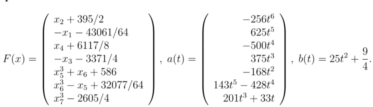
Example 4.
F (x) =
x
2+ 395/2
− x
1− 43061/64 x
4+ 6117/8
− x
3− 3371/4 x
35+ x
6+ 586 x
36− x
5+ 32077/64 x
37− 2605/4
, a(t) =
− 256t
6625t
5− 500t
4375t
3− 168t
2143t
5− 428t
4201t
3+ 33t
, b(t) = 25t
2+ 9 4 .
The algorithm output the point x = (0.9949, 0.9954, 0.9955, 0.9976, 0.9991, 0.9994, 0.9998)
⊤after 17 major iterations. The exact solution is x
∗= (1, 1, 1, 1, 1, 1, 1)
⊤.
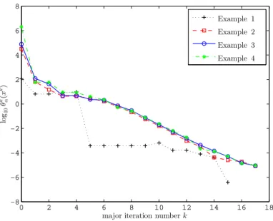
More detailed computational results are shown in Table 1 and Figure 1, where ite : the number of major iterations,
r
sum: the sum of r(k)’s, k = 1, 2, . . . , ite, where r(k) denotes the number of inner iterations within the kth major iteration,
{ r(k) } : the values of r(k) for k = 1, 2, . . . , ite,
| T
ite,r(ite)| : the number of elements of T
ite,r(ite), time(sec) : the CPU time in seconds.
In the column of { r(k) } , p q means that, for some k, we have r(k) = p in q consecutive iterations, and { p
1, . . . , p N
¯} q means that, for some k, r(k + i N ¯ + j − 1) = p j for i = 0, 1, . . . , q − 1 and j = 1, . . . , N ¯ . For example, 1
10, 3, { 1, 2 }
2means that r(1) = r(2) = · · · = r(10) = 1, r(11) = 3, r(12) = 1, r(13) = 2, r(14) = 1 and r(15) = 2. Figure 1 depicts the values of log
10θ k α (x k ) for k = 1, 2, . . . , ite.
Table 1: Computational results of Algorithm 2
Example ite r
sum{ r(k) } | T
ite,r(ite)| time(sec)
1 15 22 1
4, 2, 1
4, 4, { 2, 1 }
2, 2 9 1.41
2 17 26 1, 2
2, 1
2, 2, 1
2, 2
2, 1, 2
4, 1
211 7.05
3 17 26 1, 2
2, 1
2, { 1, 2 }
4, 2, 1, 2
211 108.25
4 17 36 4, 1, 2, 1
2, 2, 3, 1, 3, 2
3, 3, 2, 1, 4, 2 21 194.07
0 2 4 6 8 10 12 14 16 18
−8
−6
−4
−2 0 2 4 6 8
major iteration numberk log10θk α(xk)
Example 1 Example 2 Example 3 Example 4