Society of Japan
2009, Vol. 52, No. 1, 1-10
A NEW PROJECTION-TYPE ALTERNATING DIRECTION METHOD FOR MONOTONE VARIATIONAL INEQUALITY PROBLEMS
Sun Min
Zaozhuang University
(Received October 18, 2007; Revised August 29, 2008)
Abstract In this paper, we design a new projection-type alternating direction method which is an attractive method for solving variational inequality problems, and its application range covers linear programming, semidefinite programming etc. In each iteration, it just solves a linear equation and implements three orthogonal projections to closed convex sets. Under the conditions of monotonicity and Lipschitz continuity of f (x) involved in the variational inequality problems, we prove the global convergence of the new method.
Keywords: Optimization, alternating direction method, variational inequality prob-lems, Lipschitz continuous, global convergence
1. Introduction
Let S ⊂ Rn be a nonempty closed convex subset and let f be a continuous, monotone mapping from Rn into itself. Throughout the paper, we discuss the variational inequality problem: to find a vector x∗ ∈ S, such that
(x − x∗)>f (x∗) ≥ 0 ∀x ∈ S . (1.1) We use VI(f, S) to denote the above problem. VI(f, S) covers linear programming by setting f = c, a constant vector, and S = {x ∈ Rn : Ax = b, x ≥ 0}. This problem has several important applications in many fields, such as linear programming, semidefinite programming, network economics, traffic assignment, game theoretic problems, etc.[1,2,3].
There are many methods for VI(f, S). Among these methods, the projection type meth-ods are attractive for their simplicity and efficiency, especially when the feasible set S has some special structure (e.g., S is the nonnegative orthant, or more generally, a box). Most recently, Han[4] proposed an efficient alternating direction method for cocoercive nonlinear variational inequality that
S = {x ∈ Rn|Ax = b, x ∈ X},
where A ∈ Rm×n,b ∈ Rm, and X is a simple closed convex subset of Rn. In [5], Han proposed a proximal decomposition algorithm for a special form of VI(f, S) where S has the following structure:
S = S1 = {x ∈ Rn|Ax = b, x ≥ 0},
or
S = S2 = {x ∈ Rn|Ax ≥ b, x ≥ 0}.
In [5], by introducing a Lagrange multiplier y ∈ Rm to the linear constraint Ax = b, Han obtained an equivalent form of (1.1) for the special S (denoted by VI(F ,Ω)): find u ∈ Ω such that
where u = Ã x y ! , F (u) = Ã f (x) − A>y Ax − b ! , Ω = X × Rm.
In [5], the proximal decomposition algorithm searches the solution of (1.2) by an iterative method. At each iteration, it solves a system of linear equations approximately and executes a projection step to generate a temporary point, and then uses the current point and the temporary point to produce a descent direction and a step-size. The methods of Han[4,5] are attractive for their simplicity since each iteration requires only one projection to a simple convex set (or a linear equation) and some function evaluations. It would be beneficial to extend the approach[4,5] to more general VI(F ,Ω) which has been studied in [6], that is, find u ∈ Ω such that
(u − u∗)>F (u∗) ≥ 0, ∀u ∈ Ω, where u = Ã x y ! , F (u) = Ã f (x) − A>y Ax − b ! , Ω = X × Y , X ⊆ Rn and Y ⊆ Rm be given simple nonempty closed convex subset. Obviously, the variational inequality problems discussed in [4,5] are special cases of the above VI(F ,Ω). VI(F, Ω) has attracted much attention not only from optimization community, but also from application fields, because its numerous applications in operations research, economics, transportation equilibrium and so on can be explained by this model[1,3]. When X and Y are simple closed convex sets, the computational load of projection is tiny, which makes projection-type alternating direction method applicable in practice.
Note that the above VI(F ,Ω) can be expressed as follows, which is denoted by VI(Q, W )[6]: find a point w∗ ∈ W such that
(w − w∗)>Q(w∗) ≥ 0 ∀w ∈ W , (1.3) where w = x y z , Q(w) = f (x) − A>y z Ax − z − b
, W = X × Y × Rm. To solve VI(Q, W ), Wang
et. al.[6] proposed a decomposition method, but Han mentioned in [4], obtaining an exact solution of the subproblem included in [6] itself is difficult.
Using the iteration technique in [5], we propose a new alternating direction method for VI(Q, W ). At each iteration, the new method only has to solve a system of linear equation and perform three projections. The step-sizes are bounded away from zero if the mapping
f (x) is Lipschitz continuous.
The paper is organized as follows. In Section 2, we summarize some basic definitions and properties used in this paper, then we formally propose the new alternating direction, and the global convergence of the method is proved under the condition that f is Lipschitz continuous on X. In Section 3, we report some preliminary computational results of the proposed method. Section 4 gives some concluding remarks.
2. Algorithm and Convergence
We first give some basic properties and related definitions used in this paper. We denote
k · k and h·i as the Euclidean norm and inner product, respectively. We use PW(·) to denote the orthogonal projection mapping from Rn+2m onto W , that is
PW(w) = PW x y z = PX(x) PY(y) z , w = (x, y, z) ∈ Rn+2m.
It is well known that VI(Q, W ) is equivalent to the projection equation
w = PW[w − βQ(w)], where β is an arbitrary positive constant[3,4]. Let
e(w, β) = e1(w, β) e2(w, β) e3(w, β) = w − PW[w − βQ(w)] = x − PX[x − β(f (x) − A>y)] y − PY[y − βz] β(Ax − z − b)
denote the residual function of the projection equation. VI(Q, W ) is equivalent to finding a zero point of e(w, β)[3,4]. For the closed convex set W , a basic property of the projection mapping PW is
(w − PW(w))>(v − PW(w)) ≤ 0, ∀w ∈ Rn+2m, ∀v ∈ W. (2.1) From (2.1) and the Cauchy-Schwartz inequality we can see that the projection operator PW is nonexpansive, namely
||PW(v) − PW(w)|| ≤ ||v − w||, ∀v, w ∈ Rn+2m. We need the following definitions concerning the functions.
Definition 2.1.
(a) A mapping f : Rn → Rn is said to be Lipschitz continuous if there exists a constant L > 0 such that
||f (x) − f (y)|| ≤ L||x − y||, ∀x, y ∈ Rn. (b) A mapping f : Rn→ Rn is said to be monotone if
(x − y)>(f (x) − f (y)) ≥ 0, ∀x, y ∈ Rn.
In the paper we always assume that the underlying function f (·) is Lipschitz continuous and monotone, and that the solution set of VI(Q, W ), denoted by W∗, is nonempty.
We are now in the position to describe our method formally. Algorithm 2.1
Step 0. Choose an arbitrary point w0 = (x0, y0, z0) ∈ W , and set a small number ε > 0
for the solution accuracy, σ ∈ (0, 1), 0 < β < min{1, 2σ2, 1/(L + kAk2/2)},where kAk =
max{kAxkkxk |kxk 6= 0}. Set k:=0.
Step 1. Find ¯zk by solving the following system of linear equations
σ(Axk− ¯zk− b) + (¯zk− zk) = 0. (2.2) Step 2. Set ¯ yk = PY[yk− β ¯zk], (2.3) ¯ xk= P X[xk− β(f (xk) − A>y¯k)]. (2.4) If kwk− ¯wkk2 ≤ ε, then stop. Step 3. Set g(wk) = xk− ¯xk+ β(f (¯xk) − f (xk)) + σ2A>(Axk− zk− b)/(1 − σ)2 yk− ¯yk+ β(A¯xk− ¯zk− b) −σ2(Axk− zk− b)/(1 − σ)2 . (2.5)
Then compute αk by
αk = (1 − τ )kwk− ¯wkk2/kg(wk)k2, (2.6) where τ is a parameter which will be specialized later.
Step 4. Compute wk+1 = (xk+1, yk+1, zk+1) via wk+1 = P
W[wk− αkg(wk)]. (2.7)
Set k := k + 1 and goto Step 1.
First, we consider the stopping criteria in Step 2.
Lemma 2.1. For any β > 0, we have kwk− ¯wkk2 = 0 ⇐⇒ ke(wk, β)k = 0. Proof. If kwk− ¯wkk2 = 0, then
xk= ¯xk, yk= ¯yk, zk= ¯zk. By zk = ¯zkand (2.2), we have: Axk−zk−b = 0, i.e. e
3(wk, β) = 0. By xk = ¯xkand yk = ¯yk,
(2.3) and (2.4) indicate e1(wk, β) = 0 and e2(wk, β) = 0,respectively. Thus, ke(wk, β)k = 0.
If ke(wk, β)k = 0, then we have Axk − zk − b = 0 and P
Y[yk − βzk] = yk, PX[xk− β(f (xk) − A>yk)] = xk. By (2.1), we have ¯ zk− zk= −σ(Axk− zk− b)/(1 − σ) = 0. By (2.2), we have ¯ yk= P Y[yk− β ¯zk] = PY[yk− βzk] = yk. By (2.3), we have ¯ xk = P X[xk− β(f (xk) − A>y¯k)] = PX[xk− β(f (xk) − A>yk)] = xk. Thus, kwk− ¯wkk2 = 0. Q.E.D.
We thus can use kwk− ¯wkk as a measure to evaluate how far wk leaves from the solution set of VI(Q, W ). Therefore the stopping criterion in Step 2 is reasonable.
Theorem 2.1. Suppose that f (x) is monotone and Lipschitz continuous with a constant modulus L > 0, {wk} and { ¯wk} are the sequences generated by the above algorithm. Let w∗ be an arbitrary solution of VI(Q, W ). Then, we have
(wk− w∗)>g(wk) ≥ (1 − τ )kwk− ¯wkk2, (2.8)
where τ ∈ (0, 1) is a parameter in (2.6).
Proof. By the property (2.1) of the projection and x∗ ∈ X, y∗ ∈ Y , we have
(yk− β ¯zk− ¯yk)>(¯yk− y∗) ≥ 0, (2.9) {xk− β(f (xk) − A>y¯k) − ¯xk}>(¯xk− x∗) ≥ 0. (2.10) Since w∗ is the solution of VI(Q, W ) and Lemma 2 in[7], we have
(¯xk− x∗)>(f (x∗) − A>y∗) ≥ 0, (2.11) (¯yk− y∗)>z∗ ≥ 0, (2.12)
Ax∗− z∗− b = 0. (2.13) By the monotonicity of f , we have
(f (¯xk) − f (x∗))>(¯xk− x∗) ≥ 0. (2.14) Computing (2.10)+β(2.11)+β(2.14) leads us to {xk− β(f (xk) − f (¯xk)) + βA>(¯yk− y∗) − ¯xk}>(¯xk− x∗) ≥ 0, i.e., (xk− x∗)>(xk− ¯xk) + β(¯xk− x∗)>A>(¯yk− y∗) + β(¯xk− x∗)>{f (¯xk) − f (xk)} ≥ kxk− ¯xkk2. (2.15) Computing (2.9)+β(2.12), we have (yk− y∗)>(yk− ¯yk) − β(¯yk− y∗)>(¯zk− z∗) ≥ kyk− ¯ykk2. (2.16) By (2.13)+(2.15)+(2.16), we have à xk− x∗ yk− y∗ !>à xk− ¯xk+ βf (¯xk) − βf (xk) yk− ¯yk+ β(A¯xk− ¯zk− b) ! ≥ ° ° ° ° ° xk− ¯xk yk− ¯yk ° ° ° ° ° 2 − β(xk− ¯xk)>{f (xk) − f (¯xk)} −β(¯yk− yk)>(A¯xk− ¯zk− b). (2.17)
On the other hand, by the equalities (2.2) and (2.13), we have (1 − σ)2k¯zk− zkk2/σ2 = kAxk− zk− bk2 = (Axk− zk− Ax∗+ z∗)>(Axk− zk− b) = (xk− x∗)>A>(Axk− zk− b) − (zk− z∗)>(Axk− zk− b). (2.18) By (2.2) again, we have β(¯yk− yk)>(A¯xk− ¯zk− b) ≤ βk¯yk− ykkkA¯xk− ¯zk− bk ≤ βkAkk¯yk− ykkk¯xk− xkk + βk¯yk− ykkk¯zk− zkk/σ ≤ βk¯yk− ykk2+ βkAk2k¯xk− xkk2/2 + βk¯zk− zkk2/2σ2. (2.19)
where the last equality is deduced by 2ab ≤ a2+ b2. From (2.17)−σ2(2.18)/(1 − σ)2 and the
Lipschitz continuity of f , we have
(wk− w∗)>g(wk) ≥ kwk− ¯wkk2− βLkxk− ¯xkk2
− β(¯yk− yk)>(A¯xk− ¯zk− b), then from (2.19), we can get
(wk− w∗)>g(wk) ≥ kwk− ¯wkk2− β(L + kAk2/2)kxk− ¯xkk2
− βk¯yk− ykk2− βk¯zk− zkk2/2σ2.
(wk− w∗)>g(wk) ≥ (1 − τ )kwk− ¯wkk2.
Q.E.D. From Theorem 2.1, −g(wk) is a descent direction of the function 1
2||wk− w∗||2 whenever
wk ∈ W is not a solution of VI(Q, W ).
In the following, we assume that the Algorithm generates an infinite sequence. Theorem 2.2. Suppose that the conditions in Theorem 2.1 hold, then
(a). ∃ε > 0, such that αk≥ ε, ∀k ≥ 0.
(b). The two sequences {wk} and { ¯wk} generated by the algorithm are bounded. (c). lim
k→∞kw
k− ¯wkk = 0. Proof. (a). From (2.2) we have
σ(Axk− ¯zk− b) = −(¯zk− zk). (2.20)
The first part of g(wk) can be rewritten as
xk− ¯xk+ β(f (¯xk) − f (xk)) + σ2A>(Axk− zk− b)/(1 − σ)2
= (xk− ¯xk) + β(f (¯xk) − f (xk)) + σ2A>(Axk− ¯zk− b)/(1 − σ)2
+σ2A>(¯zk− zk)/(1 − σ)2.
then by (2.20) and the Lipschitz continuity of f , we have
kxk− ¯xk+ β(f (¯xk) − f (xk)) + σ2A>(Axk− zk− b)/(1 − σ)2k
≤ kxk− ¯xkk + βLkxk− ¯xkk + (1 + σ)σkAkkzk− ¯zkk/(1 − σ)2
≤ [1 + βL + (1 + σ)σkAk/(1 − σ)2]kwk− ¯wkk. The second part of g(wk) can be rewritten as
yk− ¯yk+ β(A¯xk− ¯zk− b) = yk− ¯yk+ β[A(¯xk− xk) + Axk− ¯zk− b],
then by (2.20) again, we have
kyk− ¯yk+ β(A¯xk− ¯zk− b)k
≤ kyk− ¯ykk + β(kAkk¯xk− xkk + k¯zk− zkk/σ) ≤ (1 + βkAk + β/σ)kwk− ¯wkk.
Similarly, the third part of g(wk)
k − σ2(Axk− zk− b)/(1 − σ)2k ≤ (σ + σ2)kwk− ¯wkk/(1 − σ)2.
From the above analysis and (2.6), it is easy to deduce that (a) holds.
(b). Let w∗ = (x∗, y∗, z∗) be an arbitrary solution of VI(Q, W ). By (2.7),w∗ ∈ W and the nonexpansive of the projection operator, we have
kwk+1− w∗k2 ≤ kwk− w∗− α kg(wk)k2 = kwk− w∗k2− 2αk(wk− w∗)>g(wk) + α2kkg(wk)k2 ≤ kwk− w∗k2− 2αk(1 − τ )kwk− ¯wkk2+ αk(1 − τ )kwk− ¯wkk2 = kwk− w∗k2− α k(1 − τ )kwk− ¯wkk2 ≤ kwk− w∗k2− ε(1 − τ )kwk− ¯wkk2.
Because τ ∈ (0, 1), from the above inequality, we have kwk+1− w∗k ≤ kwk− w∗k ≤ ... ≤ kw0− w∗k. (2.21) and ∞ X k=0 kwk− ¯wkk2 < lim N →∞ 1 ε(1 − τ )(kw 0− w∗k2− kwN − w∗k2) ≤ 1 ε(1 − τ )kw 0− w∗k2 < +∞.
Thus {wk} and { ¯wk} are bounded.
(c). We can get assertion (c) immediately fromP∞k=0kwk− ¯wkk2 < +∞. Q.E.D.
Theorem 2.3. Suppose that the conditions in Theorem 2.1 hold, then the whole sequence
{wk} generated by the algorithm converges to a solution of VI(Q, W ) globally.
Proof. It follows from Theorem 2.2 that {wk} is bounded, thus it has at least one cluster point. Let w∗ = (x∗, y∗, z∗) be a cluster of {wk} and {wkj} be the corresponding subsequence
converging to w∗.
Taking limit in (2.2),(2.3),(2.4) along the subsequence and using the continuity of f and the projection operator PX and PY, we have
Ax∗− z∗− b = 0, y∗ = P
Y[y∗− βz∗],
x∗ = PX[x∗− β(f (x∗) − A>y∗)],
which mean that w∗ ∈ W is a solution of VI(Q, W ). In the following we prove that the sequence {wk} has exactly one cluster point. Assume that ˆw is another cluster point of {wk}. Then we have
δ := kw∗− ˆwk > 0.
Because w∗ is a cluster point of the sequence {wk}, there is a k
0 > 0 such that
kwk0 − w∗k ≤ δ
2.
On the other hand, since {kwk − w∗k} is monotonically non-increasing (since (2.21) and that w∗ is a solution of VI(Q, W )), we have kwk− w∗k ≤ kwk0 − w∗k for all k ≥ k
0, and it
follows that
kwk− ˆwk ≥ kw∗− ˆwk − kwk− w∗k ≥ δ
2, ∀k ≥ k0,
which contradicts the fact that ˆw is a cluster point of {wk}. This contradiction assures that the sequence {wk} converges to its unique cluster point wk, which is a solution of VI(Q, W ). Q.E.D.
3. Preliminary Computational Results
First, we discuss how to estimate the Lipschitz constant L of f (x). There are some estimates
Lk for the Lipschitz constant L[8]:
Given L0 > 0,in the kth iteration we can take the Lipschitz constant as
Lk = max{Lk−1, kf (xk) − f (xk−1)k/kxk− xk−1k}, k = 1, 2, · · · , or
Lk = max{Lk−1, (f (xk) − f (xk−1))>(xk− xk−1)/kxk− xk−1k}, k = 1, 2, · · · .
We implemented Algorithm 2.1 in Matlab and tested it on a PC. The constraint set S and the mapping f are taken respectively as
S = {x ∈ R5|X5
i=1
xi ≥ 10, xi ≥ 0, i = 1, 2, ..., 5} and
f (x) = Mx + ρ arctan(x − 2) + q,
where M is a 5 × 5 matrix whose entries are randomly generated in the interval (−1, 1) and arctan(x−2) = (arctan(x1−2), arctan(x2−2), · · · , arctan(x5−2))
0
. The parameter ρ is used to vary the degree of asymmetry and nonlinearity, and q ∈ R5 is generated from a uniform
distribution in the interval (−500, 500). Other parameters used in the algorithm are set as
σ = 0.75; β = 0.2; τ = 0.3. We choose ||wk − ¯wk|| ≤ 10−6 as the stop criterion. Table 1 gives the numerical results by Algorithm 2.1 with different initial point, where TOTAL is the total CPU time , PROJ is the CPU time occupied by the projections, and I.P. denotes the initial point, Iter. denotes the iteration number when the algorithm terminates.
Table 1: Numerical results for different initial point
I.P. Iter. TOTAL(s) PROJ(s) ||wk− ¯wk||
(2,0,0,0,0) 25 0.12 0.03 2.12×10⁻⁷
(10,0,0,0,0) 32 0.18 0.04 2.53×10⁻⁷
(0,2.5,2.5,2.5,2) 22 0.11 0.03 1.80×10⁻⁸
The results in the Table 1 indicate that the new alternating direction method is available. Though the iterative number is large, the total TOTAL time is small. The reason is that at each iteration the algorithm needs not to execute linear search and only need to make some projections and function evaluations. PROJ indicates that the CPU time occupied by projections is nearly one forth of the total CPU time, and this is acceptable.
To show the advantage of the new alternating direction method for large scale problems, we implement it to a set of spatial price equilibrium problems. The details of these problems can be found in [5], as follows:
min m X i=1 n X j=1 (cijxij + 1 2hijx 2 ij). s.t. n X j=1 xij = si, i = 1, 2, · · · , m,
m
X
i=1
xij = dj, j = 1, 2, · · · , n, xij ≥ 0.
where si is the supply amount on the ith supply market, i = 1, · · · , m and dj the demand amount on the jth demand market, j = 1, · · · , n. cij ∈ (1, 100), hij ∈ (0.005, 0.01), sj and dj are generated randomly in (0, 100) for all i = 1, · · · , m and j = 1, · · · , n, and the other parameters are set as the first example. The initial point w0 = 0 and stopped for some
prescribed ε > 0. The computational results are given in Table 2 for some m and n.
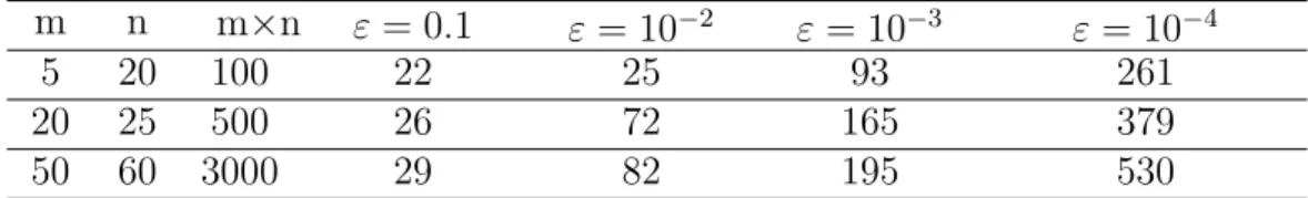
Table 2: Number of iterations for different scale and precisions
m n m×n ε = 0.1 ε = 10−2 ε = 10−3 ε = 10−4
5 20 100 22 25 93 261
20 25 500 26 72 165 379
50 60 3000 29 82 195 530
The numerical results given in Table 2 show that the new alternating direction method is relatively efficient, and it is attractive from a computational point of view.
4. Conclusion
In this paper, we proposed a new projection-type alternating direction method for monotone VI(Q, W ). The new method is easy to execute and the generated step-sizes are bounded away from zero. Under the Lipschitz continuity and monotonicity of f , we proved the global convergence of the method. Some preliminary computational results illustrated the efficiency of the algorithm.
Acknowledgements The author would like to thank two anonymous referees for their valuable suggestions and comments, which improved this paper greatly.
References
[1] D.P. Bertsekas and E.M. Gafni: Projection method for variational inequalities with applications to the traffic problem. Mathematical Programming Study, 17 (1987), 139– 159.
[2] S. Dafermos: Traffic equilibrium and variational inequalities. Transportation Science, 14 (1980), 42–54.
[3] C.H. Ye and X.M. Yuan: A descent method for structured monotone variational inequal-ities. Optimization Methods and Software, 22 (2007), 329–338.
[4] D.R. Han: A modified alternating direction method for variational inequality problems.
Applied Mathematics and Optimization, 45 (2002), 63–74.
[5] D.R. Han: A proximal decomposition algorithm for variational inequality problems.
Journal of Computation and Applied Mathematics, 161 (2003), 231–244.
[6] S.L. Wang and L.Z. Liao: Decomposition method with a variable parameters for a class of monotone variational inequality problems. Journal of Optimization Theory and
Application, 109 (2001), 415–429.
[7] B.S. He and Y. Hai: Some convergence properties of a method of multipliers for linearly constrained monotone variational inequalities. Operations Research Letters, 23 (1998), 151–161.
[8] Z.J. Shi and J. Shen: Convergence of PRP method with new nonmonotone line search.
Applied Mathematics and Computation, 181 (2006), 423–431.
Sun Min
Department of Mathematics and Information Science Zaozhuang University
Bei’an Road 1, Shandong 277160, China E-mail: [email protected]