ロジスティック回帰に基づくテスト環境要因を考慮したソフトウェア信頼性評価に関する一考察 (不確実・不確定性の下での数理意思決定モデルとその周辺)

ロジスティック回帰に基づくテスト環境要因を考慮した

ソフトウェア信頼性評価に関する一考察

On SoftwareReliabilityAssessment Based

on

Logistic Regression

with Testing Environmental Factors

鳥取大学・大学院工学研究科 井上真二，山田 茂

Shinji InoueandShigeru Yamada

GraduateSchool of Engineering,

TottoriUniversity

1

Introduction

Asoftware reliability model[11, 13] is known

as

mathematical tool forquantitativeassessment of

soft-ware

reliability. In

an

actual software testing-phase, it must be natural toconsider thatthesoftware

relia-bility growth process dependsonthetesting-environmental factors, such

as

testing-coverage,the number

oftest-runs, and the debuggingskill, which affect the software failure-occurrenceor fault-detection

phe-nomenon.

In the continuous-time software reliability modelingscheme, atesting-environmentdependent

software reliability model has been proposed by the literature [4] In the discrete-time domain, Shibata

et al. [12] andOkamuraet al. [10] proposed extended cumulative Bernoulli trial process models by

con-sidering the software metrics in software reliability assessment. On the other hand, the discrete-time

models alsohavebeenproposedby [12], [10], and [8] onlyin cumulative Bernoulli trial process modeling

approach [2].

Inthis research,weconsiderthesoftwarecomplexitywhich is measured by the number of program size

intosoftware reliability assessment. Concretely,

we

extendthe discrete program-size dependentsoftware

reliabilitymodelfollowing

a

discrete-time binomial

process [5] forincorporating

the

effect of the

testing-environmental factors into the quantitative software reliability assessment and for flexibly depicting a

softwarereliability growth

curve

describedbyobservedfaultcountingdata. Further,

we

assume

that the

discrete software failure-occurrence time distribution basically followsadiscrete Weibulldistribution for

flexibly describing the software failure-occurrencephenomenon, and considertherelationship between the

probabilitythatasoftware failure caused byafaultis observed per the i-th testing-period and the related

testing-environmentalfactors by usinga logistic regression modelingapproach. This paper alsodiscuss

parameter estimation method of

our

model proposed in this paper. Further,

we

conduct goodness-of-fit

comparisonsofourmodel with the existingcorrespondingmodel.

2

Binomial-Type

Software

Reliability Model

A discrete binomial-type software reliability model [5] is developed based

on

the following basic

as-sumptions:

(A1) Whenever asoftware failure is observed, the fault which caused it will be detectedimmediately,

andnonewfaults are introducedin the fault-detectionprocedure.

(A2) Eachsoftware failureoccursat independently and identicallydistributed randomtimes$I$withthe

discrete probability distribution$P(i) \equiv Pr\{I\leq i\}=\sum_{k=0}^{i}p_{I}(k)(i=0,1,2, \cdot\cdot$ _where$p_{I}(k)$ and

$Pr\{A\}$represent theprobability

mass

functionfor $I$ andthe probability of event$A$, respectively.

Now, let $\{N(i), i=0, 1, \}$ denote a discrete stochastic process representing the number of faults

detected up to the i-th testing-period. From the assumptions above, we have the probability mass

function that$m$faultsaredetected up to the i-th testing-period

as

$P_{f}\{N(i)=m\}=\sum_{n}(\begin{array}{l}nm\end{array})\{P(i\rangle\}^{m}\{2-P(i)\}^{n-m}p_{\gamma}\{N_{0}=n\}$ $(m=0,1,2, \cdots , n)$

.

(1)

In Eq. (1),weconsider thecasethat the probability distribution of the initial faultcontent, $N_{0}$, follows

abinomial distribution withparameters $(K, \lambda)$ whichis given

as

$Pr\{N_{0}=n\}=(\begin{array}{l}Kn\end{array})\lambda^{n}(1-\lambda\rangle^{K-n} (0<\lambda<1;n=0,1, \cdots, K)$. (2)

Eq. (2) hasthefollowingphysical assumptions:

(a) The software system consistsof$K$ linesof code (LOC) atthe beginning of the_testing-:)hase.

(b) Each code has

a

faultwith

a

constantprobability$\lambda.$

(c) Eachsoftware failure caused by afaultremaining in the software system

occurs

independently and randomly.

These assumptions

are

useful to apply a binomial distribution to the probability

mass

functionof the

initialfault content inthe softwaresystem, andto incorporatethe effectofthe programsize intosoftware

reliability assessment [7]. Theprogramsizeis

one

of theimportantmetrics of software complexity which

influences$ti_{1}e$ software reliability growth process in the tegting-phase.

SubstitutingEq. (2) into Eq. (1),we

can

derive theprobabilitymassfunction of thenumber of faults

detected uptothe i-th testing-period as

$P\mathfrak{r}\{N(i)=m\}=\sum_{n\simeq m}^{K}(\begin{array}{l}nm\end{array})\{P(i)\}^{m}\{1-P(i)\}^{n-m}(\begin{array}{l}Kn\end{array})\lambda^{n}(1-\lambda)^{K-n}$

$= (\begin{array}{l}Km\end{array})\{\lambda P(i)\}^{m}\sum_{n=m}^{K}(\begin{array}{l}K-mn-m\end{array})\{\lambda(1-P(i)\rangle\}^{n-m}(1-\lambda)^{K-n}$

$=(\begin{array}{l}Km\end{array})\{\lambda P(i)\}^{m}\{1-\lambda P(i)\}^{K-m} (m=0,1,2, \cdots K)$. (3)

FromEq. $(3\rangle$, severaltypes of discrete software reliability model with the effectofprogram size

can

be

developed by giving suitable probability distributio})$s$ for the software failure-occurrence times,

respec-tively.

3

Discrete Software

Failure

Occurrence

Time

Distribution with

TE

For flexiblediscrete softwarereliability growth modeling, weapply

a

discrete Weibull distribution [9]

tothesoftware failure-occurrencetime distribution, which is given by

$P(i)=1-(1-p_{i})^{i^{\gamma}})$ ₍₄₎

where $p_{i}$ represents the probability that a software failure caused by

a

fault is observed per the i-th

testing-period,and$\gamma$denotestheshape$i$)arameter. Thediscrete Weibull distribution subsumes geometric

and Rayleigh distribution as the special

cases.

In this research,

we

assume

that $p_{i}$ depends on the

testing-environmentalfactors at the i-th testing-period and the relationshipbetween$p_{i}$ andthe

testing-environmental factors

can

begiven by

In

Eq.

(5),$\beta_{i}=(1,\beta_{1,i},\beta_{2,i}, \cdots , \beta_{n,i})$ represents

the

$n$

kinds of

testing-environmental

factors

at

the i-th

testing-period,$\alpha=(\alpha_{0},\alpha_{1}, \cdots,\alpha_{n})$ is the coefficientvector,and$A^{T}$the transposed

matrixof thematrix

$\mathcal{A}.$

4

Software Reliability Assessment Measures

We can derivesoftware reliabilityassessment

measures

under thebasic assumptionson the software

failure-occurrence phenomenoninEq. (1). The expectationofthe number ofdetectedfaults, $E[N(i)]$, is derived

as

$E[N(i)]=\sum_{z=0}^{n}z\sum_{n}(\begin{array}{l}nz\end{array})\{P(i)\}^{z}\{1-P(i)\}^{n-z}\cdot Pr\{N_{0}=n\}$

$=E[N_{0}]P(i)$ ₍₆₎

Anditsvariance,$Var[N(i)]$, is alsoderived

as

$Var[N(i)]=E[N(i)^{2}]-(E[N(i)])^{2}$

$=Var[N_{0}]\{P(i)\}^{2}+E[N_{0}]P(i)\{1-P(i)\}$ (7)

A discrete software reliability function is defined

as

the probability that a software failure does not

occur

in the time-interval $(i,i+h](i, h=0,1,2, \cdots)$ given that the testing

or

the operation has been

going up tothe i-th testing-period. Then, the discrete softwarereliability function, $R(i, h)$, under the

basic assumptionin Eq. (1) is derived

as

$R(i, h)= \sum_{k}Pr\{N(i+h)=k|N(i)=k\}Pr\{N(i)=k\}$

$= \sum_{k}[\{P(i)\}^{k}\{1-P(i+h)\}^{-k}\sum_{n}(\begin{array}{l}nk\end{array})\{1-P(i+h)\}^{n}\cdot Pr\{N_{0}=n\}].$

(8)

Concretely,we canderive the discrete softwarereliabilityfunctioninthe

case

thattheinitial fault content

follows the binomial distribution in Eq. (2)

as

$R(i, h)= \sum_{z=0}^{K}Pr\{N(i+h)=k|N(i)=k\}(\begin{array}{l}Kz\end{array})\{\lambda P(i)\}^{z}\{1-\lambda P(i)\}^{K-z}$

$= \sum_{z=0}^{K}[\{P(i)\}^{z}\{1-P(i+h)\}^{-z}\cdot\sum_{n=0}^{K}(\begin{array}{l}nz\end{array})\{1-P(i+h)\}^{n}(\begin{array}{l}Kn\end{array})\lambda^{n}(1-\lambda)^{K-n}]$

$=[1-\lambda\{P(i+h)-P(i)\}]^{K}$ ₍₉₎

further, instantaneousand cumulativeMTBFs, $MTBF_{I}(i)$and $MTBF_{C}(i)$,

are

also derived

as

$MTBF_{I}(i)=1/(E[N(i+1)]-E[N(i)])$, (10)

$MTBF_{C}(i)=i/E[N(i)]$, (11)

respectively.

5

Parameter Estimation Method

Suppose thatwehaveobserved$N$datapairs $(t_{i}, y_{1},\beta_{i})(i=0,1,2, \cdots, N)$with_{respect to}the

related data for the testing-environmentaJ factors, $\beta_{i}$

.

Thelikelihood function, $t$, for thebinomial-type

softwarereliabilitymodel, $N(i)$_,can be _derived

as

$t=Pr\{N(t_{1}\rangle=y_{1}, N(t_{2})=y_{2},$$\cdots,$$N(t_{N})=y_{N}\}$

$= \prod_{i=1}^{N}Pr\{N(t_{i})=y_{i}|N(t_{i-3})=y_{i-1}\}Pr\{N(t_{1})=y_{1}\}$, (12)

by usingtheBayes’ formula and aMarkovproperty. In Eq. $(12\rangle, t_{0}=0 and y_{0}=0.$ Thus,$Pr\{N(t_{0})=$

$y_{0}\}=Pr\{N(0\rangle=0\}=1$

.

_{Theconditional}probability inEq. (12), $Pr\{N(t_{i})=y_{i}|N(t_{i-1})=y_{i-1}\}$, can

bederived

as

$Pr\{N(t_{i})=y_{i}|N(t_{i-1})=y_{i-1}\}=(\begin{array}{l}K-y_{i-1}y_{i}-y_{\dot{t}-1}\end{array})\{x(t_{i-1}, t_{i})\}^{y.-y.-1}\{1-z(t_{i-i}, t_{i})\}^{K-y:}$, (13)

where

$z(t_{i-1}, t_{i})= \frac{\lambda\{P(t_{i}\rangle-P(t_{i-1})\}}{1-\lambda P(t_{i-1})}$

.

(14)

Then,

we

can

rewrite Eq. (12)

as

$t= \prod_{i=1}^{N}(\begin{array}{l}K-y_{i-1}y_{i}-y_{i-l}\end{array})\{z(t_{i-1}, t_{i})\}^{y;-y_{i-1}}\{1-z\langle t_{i-1}, t_{i})\}^{K-y}\dot{}$, (15)

by usingEq. (13). Accordingly, the logarithmiclikelihood function

can

bederived

as

$\log l\equiv L=\log K!-\log\{(K-y_{N})!\}$

$- \sum_{\grave{x}=1}^{N}$iog$\{(y_{i}-y_{i-1})!\}+y_{N}\log A+\sum_{\prime,l=1}^{N}(y_{i}-y_{i-z})\log\{P(t_{i})-P(t_{i-\iota})\}$

$+(K-y_{N})\log\{1-\lambda P(t_{i})\}$

.

(16)

When we apply Eqs. (4) and (5) as the discrete software failure-occurrence times distribution, the

logarithmic likelihood function

can

be givenas

$L= \log K!-\log\{(K-y_{N})!\}+y_{N}\log\lambda-\sum_{i=1}^{N}\{(y_{i}-y_{i-1})!\}$

$+ \sum_{i=1}^{N}(y_{i}-y_{i-1})\log\{(1-p_{i})^{t_{\mathfrak{i}’-1-}^{\wedge}}(1-p_{i})^{t_{i}^{\gamma}}\}+(K-y_{N})\log[1-\lambda\{1-\langle 1-p_{i})^{t_{N}^{\gamma}}\}]$ , (17)

by usingEq. (16). Wehaveto estimate theparameters$\lambda,$

$\gamma$,and $\alpha$if

we

can

know theprogram size$K.$

Accordingly, we canobtain the maximum-likelihood estimates$\hat{\lambda},$

$\hat{\gamma}$, and $\hat{\alpha}$

ofthe unknown parameters

$\lambda,$

$\gamma$, and$\alpha$, respectively, bysolvingthesimultaneous likelihood functions with$\lambda,$

$\gamma$, and $\alpha$numerically.

6

Model Comparisons

Wecompare the performance of

our

model for software reliability assessment with the existing

corre-sponding model, whichdoes not consider the effect of the testing-environmental factors, by using two

data sets collected from actual software testing-phases. The data sets are respectively called DS1 and

DS2. The details ofthe data

are

shown

as

follows:

DS1 : $(t_{i}, y_{i}, c_{i})(i=1,2, \cdots , 22; t_{22}=22,y_{22}=212, c_{22}=0.9198)$ where$t_{i}$ ismeasublack

on

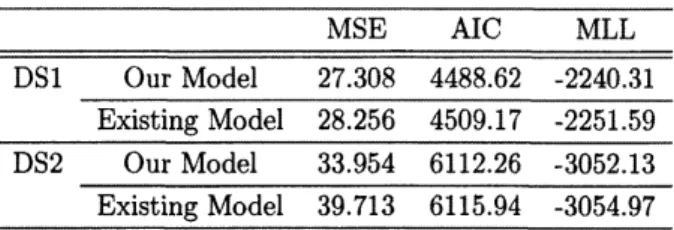
the basis

Table 1: Resultsof modelcomparisons based

on

the MSEand AIC.

$\overline{\overline{DSlOurModel27.3084488.62-2240.31}}MSEAICMLL$

$\frac{ExistingMode128.2564509.17-2251.59}{DS2OurM\circ de133.9546112.26-3052.13}$

Existing Model 39.713 6115.$94$ _$-3054.97$

DS2 : $(t_{i}, y_{i}, c_{i})\langle i=1$,2,$\cdots$ ,24; _{$t_{24}=24,$$y_{24}=296,$ $c_{24}=0.9095)$} where$t_{i}$ ismeasublack

on

thebasis

ofweeks and the programsize$K=1.972\cross 10^{5}$ _{(LOC) [3],}

where$y_{i}$ representsthe number offaults detected upto$t_{i}$ and $c_{l}$ is theCO testing-coverage attained up

to $t_{i}$

.

In this model comparisons

we

treat the CO testing-coverage

as

the testing-environmental factors

affecting the software failure-occurrence or fault-detection phenomenon. Thus, we treat that $\beta_{i}\equiv c_{t}.$

Regarding the actualdata, DS1 shows the exponentialsoftware reliability growth

curve

and DS2shows

the $S$-shaped

one.

And the existing corresponding model

assumes

that the software

failure-occurrence

time distribution follows $P(i)=1-(1-p)^{i^{\gamma}}(i=0,1,2, \cdots)$ _{in Eq. (3) [6], where} $p$ represents the

probability thatasoftware failure caused byafault is observed peronetesting-period and$\gamma$istheshape

parameter of thediscrete Weibull distribution.

Forquantitative comparisons interms of fitting performanceto the actualdata, we

use

mean square

error

(abbreviated

as

MSE) [11] andAkaike information criterion (AIC) [1]. Table 1 shows the results ofmodelcomparisonsbased onthe MSE, AIC, andMLL represents the maximum$\log$-likelihood,

respec-tively. From Table1,we cansayourmodel fits well to the actual data

even

though the actualdata shows

theexponentialor $S$-shaped software reliability growthcurve.

7

Conclusion

We proposed an extended binomial-type software reliability model with the effect of the

testing-environmentalfactorsonthesoftwarereliability growth process. Especially, the discrete software

failure-occurrencetimedistribution follows the discrete Weibull distribution basically. Further, wediscussed a

parameter estimationmethodofourmodel,and conductedcomparisonsoftheperformance of

our

model

with that of existing corresponding model in terms of MSE. In future studies, we need to check the

performance ofourmodel with existing models [8,10, 12] by using alot ofsoftware fault-counting data

with software metrics in the futurestudies because

we

have

an

enough time to obtain the appropriate

data sets and conducting numericalexperiments.

Acknowledgement

This research was supported in part by the Grant-in-Aid for Scientific Research (C), Grant No.

22510150, from the Ministry ofEducation, Culture, Sports, Science and Technology of Japan and the

TelecommunicationsAdvancement Foundation.

References

[1] H. Akaike, “A

new

look at the statistical model identification,”IEEE ffinsactions on Automatic

Control

Vol. AC-19, pp. 716-723, 1974.

[2] T.Dohi,K.YasuiandS.Osaki, “Software reliabilityassessmentmodelsbased

on

cumulative Bernoulli

[3] T. Fujiwara and$S$, Yamada, “A

new

testing-pathcoveragemeaagure-$Testing$-domainmetricsbased

on a software reliability growth model – Proc. 13th IEEE International Symposium on

Software

Reliability Engineering(ISSRE’02), pp. 71-75, 2002.

[4] $\prime\iota$

.

Imanaka and $rr$

.

Dohi, “Burr XII distribution-based software reliability modeling Proceedings

of

the 6th $\mathcal{A}sia$

-Pacific

International Symposium

on

AdvancedReliabitity and Maintenance Modeling

(APARM2014 pp. 176-183, McGraw-Hill,$Taiw^{r}an$_, 2014.

[5] S. Inoue and S. Yamada, (Generalized _{discrete softwarereliability modeling witheffect of program}

size IEEE $x\nu$ansactions

on

Systems, Man. and Cybernetics – Part $A$: Systems and Humans, Vol.

37, No. 2, pp. $170-179_{\backslash }$2007.

[6] S.InoueandS.Yamada, ((Discreteprogram-sizedependentsoftwarereliabilityassessment: Modeling,

estimation, and goodness-offit comparisons IEICE 7ransactions on Fundamentals

_of

Electronics,

Communications and Computer Sciences, Vol. E90-A,No. 12,pp. 2891-2902, 2007.

[7] M. Kimura, S. Yamada, H. Tanaka and S. Osaki “Software reliability measurement with

prior-information on initialfault content,“ Transactions

_{of Information}

Processing Society

_of

Japan, Vol.

34, No. 7, pp. 1601-1609,

1993.

[8] D. Kuwaan$d’r$

.

_{Dohi “Generalized logit-based software reliability modeling with metricsdata,”}

Pro-ceedings

_of

the 37thAnnualInternational Computer

_Software

and Applications

_Conference

(COMP-SAC 2013),pp. 246-255, IEEE CPS, 2013.

[9] T. Nakagawa and S. Osaki “The discrete Weibuh $dist_{1}\cdot$ibution,” IEEE Transactions on Reliability,

Vol. R-24, No. 5,pp. 300-301, 1975.

[1e] H. Okamura, Y. Etani and T. Dohi “A multi-factorsoftware reliabilitymodel based $oxx$ logistic

re-gression,” Proceedings

_of

the$21st$IEEE international Symposiumon

_Software

Reliability Engineering

(ISSRE’10), pp. 31-40,IEEE CPS, 2010.

[11] H. Pham, “Software Reliabi}ity,’’Springer-Verlag, Singapore, 2000.

[12] K. Shibata, K. Rinsaka and T. Dohi, “Metrics-based software reliability models using

non-homogeneousPoisson processes Proceedings

_of

The 17th International Symposium on

_Software

Re-hability Engineering (ISSRE’06), pp. S2-61,IEEE CPS, 2006.

[13] S. Yamada, “Software ReliabilityModeling –Fundamentals and Applications–,“ SpringepVerlag,