非線形競合現象における保存則と安定性 : システムの外部摂動からの回復現象

Conservation

law

and

Stability in

Competitive

Systems:

Restoration

phenomena

from external perturbation

*,1 _{Lisa Uechi and} *,2 _{TatsuyaAkutsu}

*Bioinformatics

Center, Institute

_for

Chemical Research,

Kyoto University, Gokasho, Uji, Kyoto 611-0011, Japan

[email protected] [email protected] 非線形競合現象における保存則と安定性: システムの外部摂動からの回復現象 * 上地理沙 * 阿久津達也 * 京都大学化学研究所バイオインフォマティクスセンター 数理生物情報研究領域

A conservation law and stability, recovering phenomenaand characteristic patterns of a nonlinear

dynamical systemhave been studied and applied to physical, biological and ecological systems. Inour

previous study,weinvestigateaconservation law ofasystem of symmetric$2n$-dimensional nonlinear

differentialequations. WeuseLagrangianapproachandNoether’stheoremto analyze Lotka-Volterra

typeofcompetitivesystem. We observe that the coefficients of the 2$n$-dimensional nonlinear

differ-ential equations arestrictly restricted when the system has aconserved quantity, and the relation betweenaconserved systemandLyapunovfunctionis shown in termsof Noether’s theorem. Wefind

that asystem of the$2n$-dimensional first-ordernonlinear differentialequationsin asymmetric form

should appear in abinary-coupled form ($BCF$), and a$BCF$ hasa conserved quantity if parameters satisfy certain conditions. In this paper, competitive systems describedby 2-dimensional nonlinear

dynamical ($ND$) model with external perturbations areappliedto population cyclesand recovering

phenomena of systems from microbes to mammals. Thefamous10-year cycleofpopulationdensity

of Canadianlynx and snowshoe hare is numerically analyzed. We find thata nonlinear dynamical system with a conservation law is stable and generates a characteristic rhythm (cycle) of

popula-tiondensity, which we call the standardrhythmofa nonlineardynamical system. The stability and

restoration phenomena arestronglyrelated toaconservation law and thebalance ofasystem. The

standardrhythmofpopulation densityis amanifestationof the survival of the fittestto the balance ofanonlinear dynamical system.

保存則をもつシステムの安定性、回復現象や非線形現象における固有パターンの出現は、 物理現象のみ ならず生命現象や生態系でも基礎研究やその特質についての応用がなされてきた。本研究の先行研究で は、 我々は対照的な相互作用を持つ $2n$ _{次元の非線形常微分方程式に従うシステムの保存則を導出した。} 非線形競合システムで、主に Lotka-Volterra型の競合項を含むシステムの保存則の導出にあたり、我々 はラグランジャンの手法やネーターの定理を用いた。システムが保存則を持つ場合には、$2n$_{次元の非線} 形常微分方程式に現れる係数の関係は、保存則からの制限を持つことが明らかになりシステムの保存則と Lyapunov関数と関連や、ネーターの定理からも古典的Lotka-Volterraシステムの保存量が導出できるこ とが示された。 また、対照的な$2n$_{次元一階非線形常微分方程式で記述されるシステムは}binary-coupled form $(BCF)$ で出現し、$BCF$はパラメタが保存則から導出される条件を満たす場合は保存則を持つこと が分かった。本論文では、$2n$_{次元の非線形競合システムを外部摂動項を含めた形に拡張し、 2次元の非線} 形競合モデルと外部摂動を含む保存則モデルを個体数の周期変動や外部摂動からの回復現象に応用した。 そして、Lotka-Volterra型非線形競合モデルの応用例として用いられるオオヤマネコと白ウサギの10年 周期で観測される個体密度変動に対して数値的解析を行った。我々は、保存則を持つ非線形システムは安 定性を持ち、個体数の変動に対し固有のリズムまたはサイクルを持つことが明らかとなった。我々は非線 形競合システムにおける固有のリズムを standard rhythmと呼び、安定性の一つの尺度と定義した。そし て、安定性と回復現象は保存則とシステムのバランスと強い相関があることを明らかにし、個体密度の時 間的変化に対する standardrhythmは非線形動的システムのバランスを保つための一つの適応戦略である 可能性を示した。

1

Introduction

The conceptof stability isimportantinordertounderstandnatural phenomenainphysical,biological and engineering systems. In ourpreviousstudy, we studied the relation between aconservation law and

stability of

a

$2n$-dimensional competitive systemthat contains competitive interactions, self-interactions

from

Noether’s

theorem [1]. The$2n$

-dimensional

nonlinear ordinary

differential

equations for

a

compet-itive systemconstructed to satisfy the conservation law have properties such

as

the addition law,which

is empirically interpreted

as

recovery frominjuriesof skin and tissues in biologicalbodies.

It hasbeen shown by many researchers that

a

relatively simple set of interactions

can

explain

com-plex phenomena in biologicalsystems [2, 3]. Forexample, in 1952, Turing suggested chemical molecular mechanism called the

reaction-diffusion

system [4] which is

defined

as

semi-linear parabolic partial dif-ferential equations. This

reaction-diffusion

system is well applied for explaining stripe patterns of the

marine angelfish, Pomacanthus, and restoration phenomena in its stripe pattems from injuries

was

ob-served [5, 6, 7]. Prigogine also proposedBrusselator modelwith nonlinear ordinarydifferentialequations

to illustrate spatial oscillations and Turing patterns [8]. It is also

an

interestingproblem to investigate in ecological systems if

a

large complex system

should

be

stable or

not, and

many researchers

have

dis-cussed the criteria concerningthestabilityof

a

systemfor $n$

dimensional

ordinary

differential

equations

and statistical framework [9, 10, 11, 12, 13]. What would be

a

reason

why

a

simple set of interactions

can

explain complex phenomena? We

discussed a

systemof interactions generalizing

Lotka-Volterra

type nonlinear competitive interactions and suggested that

a

conservation law could be akey to understand

complex phenomena

even

in biological and ecologicalsystems.

We investigated the system of $2n$

-dimensional

coupled first-order differential equations by using

Noether’s theorem, which led to the following results. (i) The form of differential equations and

co-efficients of nonlinearinteractions

are

strictly confined when thesystem has a conservation lawwhich is

constructed by interacting speciesof

a

particularexperimental system. (ii) The conserved quantityof

a

system produces

a

Lyapunov function whichis usually employed to studysolutions of nonlinear differen-tial equations. The conserved quantity is

constructed

byNoether’stheorem,but the analysis of Lyapunov function would be used to

check

solutions to

differential

equations including those for

non-conservative

and dissipative systems. The system ofdifferential equations with conservation law is different in this

respect. (iii) $A$ systemof interactions could be analyzed

as an

assemblyof

a

basic binary-coupledform

($BCF$_). In other words,

a

complex interacting system

can

be decomposed into

an

assembly of

binary-coupled systems. The $BCF$ system is

a

simple basic set to explain complex phenomena defined by Noether’s theorem. (iv) The$BCF$ systemwith conservation law indicates

an

addition law which

may

be interpreted

as

the restoration

or

rehabilitation phenomena; those

are

known in

a

large system of neural

network

or

computer network when

a

small disordered device

or

a

partofnetworksystem is replaced by

a

normaldevice. Theseproperties could be applied to stabilityandrestoration phenomena of biological

systems. (v) The conservation law is also useful to check accuracy of numerical solutions to nonlinear differential equations. As

summarized

above,

we

discussed that the basic nonlinear system in $BCF$ is

stable.

The binary-coupled system

and

addition law supported by

a

conservation law

can

lead

to

a

large,

stablecomplex system. Thisisanimportantconclusion on the

conserved

binary-coupledmodel. Because

the$BCF$systemhassuchseveralinteresting properties,

we

willapplythe modelinorder tostudy stability and interaction mechanisms ofbiologicalsystems.

In this paper,

we

will explain the propertiesofsolutions with

a

conservation law and applications to biological systems. InSection2,

we

extend the$BCF$model to simulate externalperturbations numerically.

There

are

various prey-predator type competitive modelswith perturbations, however, most ofthem

are

with small, stochastic perturbations. The behaviors ofconservation laws with external perturbations

have been seldom considered. We will explicitly discuss properties of the conserved, stable, 2-variable nonlinear interacting system with external perturbations and the conservation law, its indications and

possible applications to nonlinear interacting system. We will show that 2-variable $ND$ model has the

propertiesofrestoration andrecovery from externalperturbations. InSection3,stabilityandpopulation cycles of biological systems

are

examined in terms of

a

conservation law of the system. We will also

examine specific examplesof the Canadian lynxand snowshoe hare [14, 15, 16, 17, 18, 19, 20] and the

questionofpopulation cycles, andfood chainofmicrobes in thelake [21, 22]. Conclusionsandsummary ofresults

are

given inSection 4.

2

The

model of

binary-coupled

form

(

$BCF$

)

2.1

2n-

$ND$

system with perturbations

We discussed $BCF$ system and the _{conservation law} of $2n$-nonlinear dynamical (2n-$ND$) model in detail in the previous work [1]. In this study,

we

add external perturbations in $2n$-variable nonlinear

differential equations in order to examine characteristic behaviors of conserved nonlinear interacting systems. It should benoticed that the2n-$ND$model isextended by addingexternal perturbationterms which maintain a conservation law given by Noether’s theorem. The odd variable terms for $x_{i}(i=$

$1,$

$\ldots,$$2n)$

are

$d_{2k,2k-1^{\dot{X}}2k-1}= \sum_{\prime,\iota=1}^{n}\{(\alpha_{\{2ni+2k\}}+\alpha_{\{2n^{2}+2nk+2i-1\}})x_{2i-1}+(\alpha_{\{2n^{2}+2ni+2k\}}+\alpha_{\{2n^{2}+2nk+2i\}})x_{2i}$

(1)

$+\alpha_{\{4n^{2}+2ni+2k\}}x_{2i-1}x_{2i}\}\alpha_{\{4n^{2}+2nk+j\}^{X}j^{X}2k-1},$

where$k=1,$$\ldots,$$n$

.

The

even variable

terms for$x_{i}(i=1, \ldots, 2n)$

are

$d_{2k-1,2k} \dot{x}_{2k}=\sum_{i=1}^{n}\{(\alpha_{\{2ni+2k-1\}}+\alpha_{\{2nk+2i-1\}})x_{2i-1}+(\alpha_{\{2n^{2}+2ni+2k-1\}}+\alpha_{\{2nk+2i\}})x_{2i}$

(2)

$+\alpha_{\{4n^{2}+2ni+2k-1\}^{X}2i-1^{X}2i\}+\sum_{j=1}^{2n}\alpha_{\{4n^{2}+2nk+j\}}x_{j}x_{2k}+c_{2k}},$

where $\dot{x}=dx/dt$, coefficients, $d_{i,j}$ express $d_{2k,2k-1}=\alpha_{2k}-\alpha_{2k-1},$ $d_{2k-1,2k}=\alpha_{2k-1}-\alpha_{2k}$

.

The linear

$co$efficients and nonlinear $co$efficients $\alpha_{i},$ $(i=1, \ldots, 8n^{2}+2n)$

are

arbitrary constantvalues. The last

terms$c_{2k-1},$ $c_{2k},$ $(k=1, \ldots, n)$of(1) and (2)

are

constants orpiecewisecontinuous constants, whichare interpreted

as

external perturbations (temperature,

seasons

and other temporal, external inputs). One

should note that constant terms have dimension ofvelocity,

so

they

are

different from actual external perturbations which

are

considered to effectively express external perturbations. Because extemal per-turbations (inputs) changepopulationdensities as$\dot{x}=dx/dt$, wesimulate numerically thoseeffectswith

$c_{2k-1},$$c_{2k}$ asexternal inputs. The system has

a

conservation lawderived from Noether’s theoremwhich is proved inthe paper [1]:

$\Psi\equiv\sum_{i=1}^{n}\sum_{j=1}^{2n}\{\alpha_{\{2ni+j\}}x_{2i-1}x_{j}+\alpha_{\{2n^{2}+2ni+j\}}x_{2i}x_{j}+\alpha_{\{4n^{2}+2ni+j\}^{X}2i-1^{X}2i^{X}j\}}$

(3)

$+ \sum_{i=1}^{n}\{c_{2i}x_{2i-1}+c_{2i-1}x_{2i}\}.$

Therefore, with theequations from (1) to (3),

we

are

abletoconsider the conservednonlinear dynamical system with external perturbations by employing piecewise continuousconstantterms, $c_{2k-1},$ $c_{2k}.$

The physical meaning ofconserved quantities in

a

biological system is difficult to define contrary to classical mechanics in physics, and

so

we

would like to explain differences between $\Psi$-function and

Hamiltonian. The $\Psi$-function in this study is derived from Noether’s theorem with Euler-Lagrange

equations of motion applied to the 2n-$ND$ system. We discussed the binary-coupled form to generalize

The binary-coupled system has the

conserved

quantity ($\Psi$-function) and the $\Psi$-function may have

similar physical meanings

as

theHamiltonian of

a

system. However, theHamiltonian is defined

as

the

total energy of

a

system, and the energy has the dimension of the work, which is defined

as

force $\cross$ displacement [23, 24]. The

conserved

quantity$\Psi$ is constantalong with time,but it is

constructed

from

interactions of 2n-$ND$ system, not fromthe force, kinetic energy and potentialswhich are, inprinciple,

$co$nverted to theworkproducedbythesystem. Hence,the$\Psi$-function may wellbecalled

as the‘conserved

quantity’, but not

as

the Hamiltonian ofthe system. The $\Psi$-function may correspond to (generalized)

kineticand potential energies of

a

system, but it isnot possibletoprove that the$\Psi$-functionisequivalent

to

the Hamiltonian in terms

of

physics. In

the 2n-

$ND$ model,

variables

denote population densities

of a

systemof extended

Lotka-Volterra

type

differential

equations, anditis inappropriate todirectly interpret

the $\Psi$-function

as

the total energy

or

biomass of the system. However, it is important to comprehend

that the conserved $\Psi$-function controls behaviors andproperties of the system.

Weshowed that theconserved quantity, $\Psi$-function,

can

reproducetheLyapunov function of classical

Lotka-Volterra equationsintheprevious$wo$rk [1]. It is essential to understand that Lyapunov functions

for certain systems of differentialequations

can

be derived from Noether’s theorem when

a

system has

conserved quantities. Hence, in

conserved

systems such

as

2n-$ND$ systems, the conservation law and

Noether’s theorem are fundamental to study properties of the system. The system with Lyapunov function haslimit cyclesand attractors, which designateenergydissipations of thesystem. Thesystems with $\Psi$-functionsarestrictlyconserved systems, whichshouldcorrespond tolimit cycles atagiventime.

The dynamics of the system of$\Psi$-function evolvesaccordingto the conservation law $\Psi$,whichis equivalent

to Lagrangian dynamics in physical systems.

2.2

Properties of

2-variable

$ND$

model

The equationsof2-variable$ND$ model

are

produced by setting$n=1(k=1)$ in equations (1)to (3),

resulting in

$\dot{x}_{1}=\frac{1}{d_{21}}\{(\alpha_{4}+\alpha_{5})x_{1}+2\alpha_{6}x_{2}+2\alpha_{8}x_{1}x_{2}+\alpha_{7}x_{1}^{2}\}+\frac{c_{1}}{d_{21}}$, (4)

$\dot{x}_{2}=\frac{1}{d_{i2}}\{2\alpha_{3}x_{1}+(\alpha_{4}+\alpha_{5})x_{2}+2\alpha_{7}x_{1}x_{2}+\alpha_{8}x_{2}^{2}\}+\frac{c_{2}}{d_{12}}$, (5)

and the

2-variable

$ND$

model has

the following

conservation

law,

$\Psi\equiv\alpha_{3}x_{i}^{2}+(\alpha_{4}+\alpha_{5})x_{1}x_{2}+\alpha_{6}x_{2}^{2}+\alpha_{7}x_{1}^{2}x_{2}+\alpha_{8}x_{1}x_{2}^{2}+c_{2}x_{1}+c_{1}x_{2}$

.

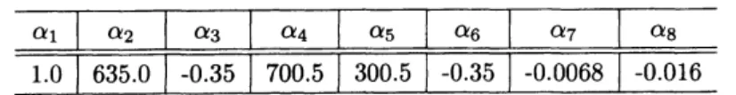
(6)

The nonlinear interactions can generally represent, for example, Lotka-Volterra type prey-predator, competitive interactions, food-chain relations by adjusting nonlinear parameters$\alpha_{1},$_$\ldots,$$\alpha_{8}$

.

The

piece-wise continuous constants, $c_{1}$ and$c_{2}$

are

used

as

externalperturbations in computer simulations,such

as

environmental conditions which increase

or

decreaseinteracting species in questions. The equations (4)

$\sim(6)$ form 2-variable$BCF$ nonlineardifferentialequations with

a

conservation law.

Byemploying eqs. (4) $\sim(6)$,

we

will show:

(1) solutions tothe binary-couplednonlinear equations maintain acharacteristic $(x_{1}, x_{2})$ phase-spaceof

solutionsandrecovery fromexternal perturbations. Theexternal perturbations

can

numerically reproduce environmental conditions suchas temperature, climate and chemicalsubstances which affect interacting

species. The nonlinear binary-coupled model

can

be applied to examine responses of

a

system whether they

are

induced from internal interactions

or

externalperturbations.

(2) The binary-coupled nonlinear equations with conservation law exhibitstable phase-space solutions,

which

are

interpretedasstability andrecovery ofpopulation-change inabiological system. The properties of the binary-coupled nonlinear interactions will be shown explicitly in numerical simulations.

(3) Byemploying the 2-variable binary-coupled model, it is possible to simulate cycles ofmaximaand

minima in population-change, delaysofperiodic times of population cycles for competitive species. Hence, cyclesof population-changewillbediscussed intermsof theconservation law and nonlinear interactions.

Time

(a) 2-variable $ND$ _solutions. Solid and dashed

lines represent $x_{1}$ (prey) and $x_{2}$ (predator),

re-spectively. One shouldnotethat theunit of time

shouldbedefined withrespecttoasystemin

con-sideration.

$x_{1}$

Time

(b) Phase-spaceof 2-variable$ND$_{solutions. (c)} Conservation law$\Psi$of 2-variable$ND$. Itis

con-stant with respect totime.

図 1: $A$ 2-variable $ND$solution and Conservationlaw $\Psi.$

Figure l(a) shows the nonlinear interactions between specieswithout external perturbations $(c_{1}=0$

and$c_{2}=0)$,whose coefficients of nonlinearequationsaresetasinTable 1 (Condition 1). Inaview of the classical Lotka-Volterra competitive system, it

can

be interpreted

as

that $x_{1}$ and $x_{2}$ represent prey and

are

periodic with respect to time, the maximum and minimum

of

$(x_{1}, x_{2})$

appear

with

a

time-delay.

Figure 1 (c) shows the numerical value of the conserved function $\Psi$definedby (6),which is constant with

respect to time.

Thesolutions $(x_{1}, x_{2})$ in Figure l(a) showexplicitly

a

time-delayof the peakfor interacting species.

The timings ofpeak and delayedpeak

are

determinedby nonlinear interactions and strength ofcoupling

constant.

The solutions $(x_{1}, x_{2})$ in Figure l(b)

show

phase-space solutions, which

are

stable

in the

meaningthat the

conserved

quantity$\Psi$ is

maintained constant

and phase-space

solutions

are

inthe

same

trajectory for alltime. The unitoftimeshould beconsidered toadjust to the time scale of

a

system in

consideration, because biological unit times

are

generally different from microbes to mammals.

Thephase-space diagram 1 (b) and thestraight lineof Figure 1(c)show that the solutionisexact and stable [1]. Thethree figures exhibit important propertiesofsolutions to thesystemof prey-predator type

ofcompetitive nonlinear interactions.

One of theimportantproperties shown by thestable,conserved nonlinear systemisthat theinteracting

species repeattherhythm of maxima and minima of thepopulation. The periods of the rhythm

are

the result ofcomplicated nonlinear interactions, but the systemkeepsthe constant quantity $\Psi$ with respect

totime. The interesting applications of the$BCF$ model

are

shown by employing in thepaper ‘Mysis in the Okanagan Lake food web ‘[21], Canadian Lynx and snowshoe hare [15], which will be explained in

Section 3.

2.3

Recovering

and restoration

from

perturbations

In order to investigate

responses

of

a

system toexternal perturbations,

we

introduce piecewise

con-tinuousconstants, $c_{1}$ and $c_{2}$, by using

$\theta$-functions such that

$c_{i}=f_{i}\{\theta(t-t_{start})-\theta(t-t_{end})\}, (i=1,2)$, (7)

where$\theta(t-t’)$ representsastep function:

$\theta(t-t’)=\{\begin{array}{l}1, (t\geq t’) ,0, (t<t’) ,\end{array}$ (8)

and coefficients $f_{i}(i=1,2)$

are

positive

or

negativeconstants to express strength of external

perturba-tions. The constants

are

adjusted to produce reasonable maxima and minimainnumerical simulations.

Figures 2(a), 2(b) and 2(c) show the reaction and recovery ofthe nonlinear interacting system from an external perturbation. One ofthe typical recoveryof

a

system froma perturbed state is shown. In

Figure 2(a), an external perturbation starts at $t=700$ (Sp. 1), and thecoefficient $f_{1}$ equals to $-1260.0$

and$f_{2}$ equals to

zero

inthis example. Theblack

arrow

isthe starting point of perturbation, and thegray

arrow

istheend ofperturbation in Figures 2(a) and 2(c). The nonlinear coefficients

are

listed inTable 1

(Condition 1). Thesolutions $(x_{1},x_{2})$

are

deformedbytheperturbation(Figure 2(a) and $2(b)$). However,

the system does not disintegrate butfinds

a new

stablephase-spaceclose totheoriginal$phasrightarrow$space and

maintains

a new

conserved relation. The perturbation endsat$t=1200$ (Ep. 1), and the system

recovers

the original state $(x_{1}, x_{2})$

.

Thetimingofnegativeperturbation

which

reduces the population number$x_{1}$

or

$x_{2}$produces different

results. Whenanegative perturbation isexertedintheincreasing phaseof$x_{1}$

or

$x_{2}$, thesystemwill find

a new conserved stable solution

near

the original solution, but when

a

negative strong perturbation is exerted before$x_{1}$ or $x_{2}$ gets to itsminimum, the system may collapse: the system exhibits nosolutions

Time

(a)2-variable$ND$_{solutions with}a negative

pertur-bationonprey$X1$. The perturbationis introduced

from$t=700$ to$t=1200$which is representedas

graybackground.

$x_{l}$

Time

(b)The$(x_{1},x_{2})$phase-spacetransitionwith the (c) Conservation law$\Psi$of 2-variable$ND$withone negativeperturbationasin(a). Solid line(St. 1) perturbation. $\Psi$changed$\Psi\simeq 60000$to$\Psi\simeq 30000$

is initialstate, andSt. 2is therecovered state by introducing perturbation. It recovers after

after the end of perturbation. Dashed line is Ep. 1.

phase-space during Sp. 1-Ep. 1.

図 2: An external perturbation anda recovery.

The conserved nonlinear system naturallyexhibits maxima and minima without external perturba-tions, and

so

we

callthese maxima and minima

as

endogenous maximumand minimum. It is needed to distinguishthemfrom enhanced maxima andminima byexternal perturbations.

In Figure 3, the response of a strong negative perturbation to prey after the peak of endogenous maximum is shown. The values ofcoefficients are listed in Table 1 (Condition 1). The starting point of this perturbation is at $t=800$ and the end point of the perturbation is at $t=950$. The negative

constant ofperturbationis $f_{1}=-3175.3879$

.

The prey, $x_{1}$, rapidlydeclines with negative perturbation,

and $(x_{1}, x_{2})$ converges to

zero

for$t>1000\sim$

.

Thesecomputersimulations may becompatiblewith known

empirical results, for example, in pest control. $A$pest controlis not

so

effective ifit is performed inthe

season

when harmfulinsects

are

in peak and active, because species

are

energetic enough to finda new

stablelife to live. It iseffectivewhenapestcontrol is performed inthe

season

whenharmful insects

are

not

so

activeor inadecliningstateafter endogenousmaximum.

In thenonlinearinteracting system, positive perturbations which will increase$x_{1}$ or$x_{2}$ donot always

mean a

positiveeffect

on

stabilityofthe system. Thereis

a

limitto the value of

a

positiveperturbation,

Time

Time

(a) 2-variable$ND$solutions with acritical neg- (b) Conservation law $\Psi$ with acritical negative

ativeperturbationon prey, $X1$. Solutions con- perturbation. $\Psi$convergestozero afterthecritical

vergetozeroafter the perturbation. perturbation.

図3: Critical negative perturbation andextinction.

system hasinternallyallowed maximum and minimum populations.

Figures 4 shows the behaviors of$(x_{1}, x_{2})$ at normal and criticalvalues of positive perturbations, $c_{1},$

for $x_{1}$

.

The values ofcoefficients

are

listed in Table 1 (Condition 2). Figures 4(a) and 4(b) show that

the normal positive perturbation which increases interacting species will increase the peak of $(x_{1}, x_{2})$

populations. However, at certain critical values of coupling constants, the prey-predator interaction cannot keep andsupportthe rhythm of maxima and minima, and the systemdiverges. Figures4(c) and

4(d) show that thesystem cannot maintain

a

stable, interactingsystem when the positiveperturbation

surpassesthe critical value ($c_{1}=1599.924999$ inthe current simulation). The unstablesolutionsbranch

out at$t\simeq 1100$ when thevalue of perturbationchanges from $f_{1}=1160.0$ to $f_{1}=1599.924999.$

Hence,in

a

conserved stablesystem, species

seem

to strictly control each other by seeking

a new

stable solution so that they can survive together. The competitive interacting system such

as

the conserved prey-predator relations

may

be

considered

to be

a

cooperative system

for

speciesto survive. It

should

be noted that if

a

dynamicalprey-predator system is active,therhythmsof maxima and minima

are

clearly

repeated, whichis known inreal prey-predator systems. However,ifan external perturbation (exogenous

interaction)exceeds a certain critical value of thecompetitive system,therhythmsof maxima andminima will disappear first and then afteratime, the system will diverge (disintegrate). Therefore, the rhythm

ofwild-life indicates that the dynamical interactions between species

are

active and stable. When the rhythm of changedisappear

or

does not

come

back, it may indicate that related species

are

in danger

of extinction. The rhythm is important toexamine if the wild life is normal and active,

or

harmed by human activities and external perturbations.

On the other hand, by adding another perturbation,

we can

show that it is possible to

save

species

from extinction. Figure 5(a) is

a

result of a positive perturbation to

save

species $(x_{1}, x_{2})$ in a danger

ofextinction in Figure 3(a). We exerted

a

positive perturbation after Sp. 1 - Ep. 1 in Figure

5.

The

positive perturbationsstart at $t=1000$ (Sp. 2) and end at $t=1300$ (Ep. 2), the strengths of$c_{1}$ and $c_{2}$

are

$f_{1}=200,$ $f_{2}=-1000$. Figure 5(a) showsthat species

are

indangerofextinction,however, ifpositive

external perturbationsare properly inserted, the systemwill

come

backto lifeagain.

2.4

Comments on “atto-fox problem”

It should be noticed that

a

problem known

as

“atto-fox problem” [25, 26] in

a

system of differential equations will not

occur

in a conserved system ofdifferential equations, because theproblem is related

$\tilde{\approx\dot{vg}}h$

$\frac{.\overline{\Leftrightarrow}}{\underline {}a}$

$a^{e}\approx\Rightarrow$

Time

Time

(a) 2-variable$ND$solutions with a _positiveper- _{(b)TheConserved quantity}$\Psi$withapositive

per-turbation. Theperturbation starts at $t=500$ turbation. Itrecoversafterperturbationbutfinds

and ends at $t=900$ represented as gray back- anotherequilibriumstate.

ground. The amplitudes of$x_{1}$ and $x_{2}$ become

larger than before.

Time

Time

(c) 2-variable$ND$ _{solutionswith a}critica] _{per- (d) Conservation law of 2-variable}$ND$_witha

crit-turbation. $x_{1}$ and$x_{2}$ convergeto zero after a ical perturbation. The$\Psi$convergestozeroaftera

critical perturbation. _criticalperturbation.

図 4: _{Critical perturbations and divergenceof solutions.}

to properties of the conserved

or

non-conserved system ofdifferential equations. The 2n-$ND$ system has the conservation law and the $\Psi$-function characterizes behaviors of solutions

and systems. If $\Psi-$

functionis conserved andnotequal to zero, Ae solutionwillconvergeand the system will be stable. The

nonlinear ordinary differentialequations with a conservation law

can

have a stable solution controlled

by the $\Psi$-function, andsolutions consist of

a

closed hyper-surface of_{$(x_{1}, x_{2}, \ldots, x_{2n})$}

for $2n$-dimensional

case.

It should be noted that the admissible coefficients of nonlinear interactions

are

strictly confined by

$\Psi$-function of the system.

The $\Psi$-function will not be constant when there

are no

solutions

or

unphysical solutions, and the property to maintain $\Psi$-function

as

constant will confine admissible

solutions [1]. For example, if the

2-variable nonlinear interacting system has solutions which areextremely different

as

$10^{-18}$ orders hke

“atto-foxproblem”, it isnot possible that thesystem

can

maintain $\Psi$-function

as

constant intime. The

phenomenon like “atto-foxproblem” would appearin dissipative

or

non-conservedsystems, because

non-conserved and dissipative systems do not have the conservation law to control admissible solutions, and

alarge class of (unphysical) solutions

can

beallowedcomparedtothe system of$\Psi$-function, which isthe

Time

Time

(a) 2-variable $ND$solutions with perturbations (b)Conservation law $\Psi$withtwoperturbations in

toavoid convergingtozero afteracritical per- (a). $\Psi$recoversfrom the perturbationafterSp. 2

turbation. $x_{1}$and$x_{2}$comebackto lifeafterthe -Ep. 2.

second perturbations.

図5: Thecriticalbehavior and restoration.

conserved systemwith $\Psi$-functionwillproduce physicalsolutions controlledbythe conservationlaw,and

the phenomenon like the

“atto-fox

problem” will not be allowed in

a

conserved systemwith $\Psi$-function.

3

Conservation law and population

cycles

3.1

The

food-web

of

Microbes in

Okanagan

Lake

One of interesting data of the ecological interactions is the interaction described in ‘Mysis in the OkanaganLake food

web: a

time-series analysis

of

interaction strengths in

an

invaded plankton

commu-nity ‘[21]. Althoughthe food-webin OkanaganLakeis not

clarified

definitely,mysis

introduction

to

lakes

isknown

as

an

effective methodtoenhance ecological interactions and its strengths

among

microbes and other creatures

so as

to increase fisheriesproductions.

The time-series of dominant crustacean zooplankton densities in Okanagan lake has been measured

monthlyand suggestedthatmysisandzooplankton populations

are

synchronousandcharacterized by the

cycleof thepeakand bottom population densities. Thecyclesofpopulation densities

are

primarilydue to

cyclesof

season

and climate and then to mutual interaction of microbes. The analysis of microbes suggests

that the density-dependent and delayed population regulationof microbesisevident. In addition to the seasonalfactors, the regular cycles and the delayed peak and bottom populations densities of microbes

are

the results of strong nonlinear interactions ofspecies. Wenumericallyexaminedchangesofpopulation densities of microbesby employingthe2-variable conserved $ND$ model.

Thecurrent

conserved

nonlinear

model

shows that the interacting species designate

a standard

rhythm of the peak and bottom population densities. There

are some

fluctuations at the peak and bottom

densities, buttheyshow the stabledynamiclife

as

demonstratedinFigure6 $(a)\sim(c)$

.

Although, normal

peak and bottom densities

can

be readily explained by adjusting coupling strength of model’s internal interactions,

a

suddenchange ofmaximawhich isoften encountered inabiological datacannot be easily simulated by onlyadjustinginternal coupling constantsinthe 2-variable nonlinear interactingmodel.

InFigure 6, several perturbations

are

exerted

on

theinteracting2-variablesystem. The first extemal

perturbation starts at $t=500$ (Sp. 1) and ends at $t=1000$ (Ep. 1). The strength ofperturbations in Sp. 1-Ep. 1

are

$f_{1}=-800,$ $f_{2}=-100$

.

The second external perturbationstarts at $t=1400$ (Sp. 2) and

Time

(a) 2-variable $ND$ _{solutions with three external}

perturbations. The rhythm of$x_{1}$ and $x_{2}$

recov-ersfrom severalperturbations. Graybackgrounds

represent periodsofperturbations.

$x_{1}$

Time

(b) Phase-space transitions of $x_{1}$ and $x_{2}$. (c) Conservationlaw$\Psi$with three perturbations.

Dashed lines represent solutions, $x_{1}$ and $x_{2}$, Itrecovers from three perturbations. $\Psi\simeq 60000$

during perturbations. Solid line represent so- in the St. 1 andSt. 2.

lutionswithout perturbations.

図6: Severalexternal perturbationsandrecoveries.

third external perturbation starts at $t=2200$ (Sp. 3) and ends at $t=2600$ (Ep. 3). The strength of

perturbations in Sp. 3-Ep.3is set

as

$f_{1}=-500,$ $f_{2}=-50$

.

Thelines$(x_{1}, x_{2})$ mayrepresentforinstance,

theprey-predator interactions, speciesof food-chain,andspeciesinteractingwith its environmentalfactors

(temperature

or

some

environmentaleffects). Black

arrows are

starting point ofperturbations, and gray

arrows are

the end ofperturbations; parameters

are

listed inTable 1 (Condition 1). The timeperiodis

within$t=4000$, initial values

are

$x_{1}=500,$ $x_{2}=300.$

The significant propertiesof the stable nonlinear conserved system arethat if external perturbations

arenot large enough to disintegrate the system, the system will find astable conserved solution nearthe original system and continuea stable cycle (maximaand minima). Itis clearlyseen from $(x_{1}, x_{2})$-phase

space solutions inFigure 6(b). Thesystem

recovers

from several externalperturbations.

The numerical analysis

can

be applied to examine the change ofpopulation densities of microbes. For example, the time-series data of dominant crustacean zooplankton densities in the Figure 2 of the

paper ‘_{Mysis in the Okanagan Lakefood-web ‘, show that the sudden maxima of dominant zooplankton}

densitiesare seen in the period $99\sim 02$

.

The sudden increaseofthe _{peak is} readily adjusted when an

couplingconstants in the

2-variable nonlinear model.

Hence,it is

concluded

in

the 2-variable model that

there would have

been

certain positive

external

perturbation to thesystemofmicrobesinOkangan Lake

during $98\sim 01$ considering atime-delayofextemal perturbations.

It is interesting tocheckwhat kindof

external or

internalperturbations is affectingthe peak of popu-lationdensity during theperiod $98\sim 01$

.

If there

are

no

explicitchanges in external

or

internal factors

duringtheperiod,

a

suddenincrease of thepeakcouldbe

a

resultof

more

complex

internal

interactions. Forexample,the rhythm of the peak

and

bottom population densities

should

be explained by

4-variable

or 6-variablenonlinear interactions of microbes. Theunusualrhythm indicates howexogenous (environ-mental) and endogenous (internal interactions) variables

are

affecting the dynamicsof each component

and environmental nature related tothe species. The analysis of nonlinear modelsuggests thatthe sud-den peak and bottom sud-densities have important information

on

the dynamics of the system

of

species

and

environment. Hence, it

is

important

to understand the standard

rhythmof

the

peak

and bottom

populationdensities inorder to distinguish them from unusual maxima andminima.

$O$

ne

should be

careful

that

a

positive perturbation

on

one

of interacting species not only enhances

the peak ofmaximabut also decreases minima intherhythmofspecies. Itisoftentrue that the effect of

enhancement is usually emphasized without taking

care

after negativeeffects. Hence, the enhancement ofthe numberof population of

a

specific species may be harmful to other species in the food-web and

consequently it endangers itself. Our analyses in Figure 4 and 5 show that if

we

carefully control the increase or decrease ofthe population ofcertain species after introduction of a positive effect,

we can

keep normal andstabledynamics of speciessuitable for theenvironment. For thispurpose, it isessential to explicitly understand the standard rhythm from real observed data.

3.2

Population regulation in Canadian

lynx

and snowshoe hare

It is difficult to identify population regulation mechanisms about prey-predator patterns of large

mammals because the large mammal’s life span is relatively long compared with microbes. The

prey-predator cycle such

as

wolves and caribous takes

some

decades of years to observe, their interacting relation and behaviors havebeen recently revealed withmoderntechnology (GPS-colored animals) [14]. However, the food-web configuration between snowshoe hare and Canadian lynx is well-known

prey-predatortypephenomena,and

a

ten-year cycle of Canadianlynx

was

examined from the data of

Canada

lynxfur-trades return ofthe NorthernDepartment of theHudson’s Bay Company (thedata

are

fromC. Elton and M. Nicholson [15]$)$

.

The Canadian lynx and snowshoe hare have a synchronous ten-year cycle in population numbers

[14, 16]. The fundamental mechanisms for thesecycles

are

maintainedbythe importantfactors such

as

nutrient,predationand social interactions [17]. Inadditiontotheimportantfactors,the nonlinear model

with conservation law suggests that species ofasystem consequently find astrategyor a mechanism to

survive for long-time periods. In other words, the cycleofpopulation density is a manifestation of the

strategy or mechanismtosurvive,whichissuggestedby stabilityofphase-space solutions determined by

conservation law ofasystem.

Thenonlinear interactions with conservation law show

a

standard rhythm andstabilityfrom external

perturbations

as

shown in Figure 6. The feeding and nutrient experiments in [17]

are

considered

as

Time

Time

(a) The2-variable $ND$simulation of Canadian _{(b) The estimated population of Canadian lynx}

lynx population. Thesolidline representsCana- and snowshoe hare. The dashed line represents

dian lynx population [15], and thedashed line Canadian lynx population simulated by 2-variable

represents a theoretical solution of 2-variable $ND$ _{model with perturbations, and the solid line}

$ND$with severalperturbations. _{represents approximate population of snowshoe}

hare.

Time

(c)Transition of conservationlaw $\Psi$with respect

to time. Severalperturbationsareintroduced.

図 7: Simulation of Canadianlynx and snowshoe hare.

external perturbations to thesystem. As shown in Figure 6,the perturbations

cause

certain effects

on

the system, but the system will find

a

rhythm to maintain the dynamics of species, which is not so different from the original standard rhythm. Our numericalresults agree with conclusions derived from feedingexperimentsand nutrient-additionexperiments. Therefore, we propose that theproperties of the

system which has a conservation law should be akey to understand the unanswered question: why do these cycles exist?.

Theresults of computersimulations showthat the timing ofperturbation leads to different results.

This isalso confirmed by the feedingexperiment of snowshoe hare: “

$\cdots$ duringthe peakofthe cycle in

1989 and 1990 had no impact

on

reproductive output $\cdots$ however, during the decline phase in 1991 and

1992, thepredator exposureplus food treatment caused a dramaticincreasein reproductive output $\cdots$

”

[17]. This fact canbe examined inourmodel calculations. The perturbation in the peak phase does not

cause large effects on standard rhythm, but negative and positive perturbations during a decreasing

or

increasing phase induce dramatic effects.

The cycle of standard rhythm forCanadianlynx and snowshoe hareindicates that the stable

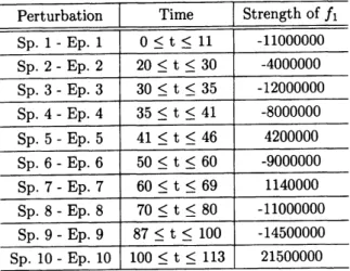
Table 3:

The list of

external

perturbations in Figure

7.

The periods of positive and negative perturbations

to numerically simulateCanadianlynx population. Note that the values of$f_{1}$ have the meaningofvelocity

(number/time).

conditions. However,

as

we have shown in Figure 4(c) and 4(d), if

a

strong negative perturbation is applied persistently for

a

long period, the system would fall into

a

dangerofextinction. The important

results of

our

simulation tellthatbefore

a

system getsin dangerofextinction,the standard rhythm of the system will

tend to

become ambiguous

or

disappear. Hence,if

we

carefullyobserve the standard rhythm of

a

specific system of species,

we

could

help the dynamical system

save

and preserve related natural

environment.

In Figure 7,

we

simulated the Canadian lynx data of the Hudson’s Bay Company from 1821 to

1910, which isapproximatelythought

as

thelynx-populationdensity. The interpolatedElton’s data

was

downloaded from [27]. The solid-line in Figure 7(a), is lynx-population dataandthe

dashed-line

is the

results of

our

numerical simulation using 2-variable nonlinear interactions between lynx and snowshoe

hare (Figure $7(b)$). The

conserved

binary-coupled model tells that there

should

havebeen

some

external

perturbations, although we cannot make

sure

atthe present what kinds of extemal perturbations

were

exerted. The actual population densityof snowshoe hare isnot known,and

so

we

assumed

a

reasonable

population density and several externalperturbations for numerical simulations inorder to fit the lynx

population data (see,Table 2 and Table3).

The

snowshoe

hare gets

several

positive and negative perturbations, but the

overall

rhythms of lynx

and hare

are

not altered. As suggested by in Figure 6(b), the phase-space

of

lynx and

snowshoe

hare

is stable against several external perturbations. This is also compatible with the empirical fact that

the ten-year cycle in snowshoe hare is resilient to a variety of natural disturbances from forest fires to short-term climaticfluctuations. However,

as

shown in

our

modelcalculationin Figure4(c), along-term

(morethanten years) negativeperturbations and a vast environmentalchangethat humans could

cause

would definitely endangerthe standardrhythmofsnowshoehare, lynx and related species.

4

Conclusions

Inthis paper,

we

examined characteristic propertiesof severalecological systemsbased

on

conserved nonlinear interactions which include generalized

Lotka-Volterra

type prey-predator, competitive

interac-tions. In Section2.1,

we

extended

our

$2n$-variable$ND$ modelby includingexternal perturbations inorder

to apply themodel to

more

realistic biological phenomenaand to study responses of

a

biologicalsystem

We simulated extemal positive and negative perturbations by employing piecewise constant terms

in

our

nonlinear equations. As it is discussed in the analysis, the results of simplified perturbations agreed with the experimentsand empirical data reasonably well. The numerical simulationsshowed the existence of the standard rhythm which ischaracteristic to

a

nonlinear conserved system. It is essential

to understand standard rhythm by observing and taking dataof a system

so

that

we

can distinguish

unusual maxima and minima fr$om$ standard rhythm This gives

a

possibility to examine signatures

that

distinguish internal effects

from

external

ones.

Theten-year cycleoflynx and hare is a very interesting biological phenomenon. Though

a

cycle of

abiological system should be aphenomenon composedofcomplex and multi-biological interactions, the 2-variable $BCF$ _{analysis has revealed the interesting results}

_on

_{properties ofthe biological phenomena.}

The ten-year cycle of lynx and hare is stable and resilient to extemal perturbations, which is

repro-duced in

our

model calculations. The system with conservation law shows stablecycles and recovering phenomena, which

are

displayed numerically in phase-space solutions. The stability and conservation law

are

constructed at least by binary-coupled species in biological and ecological systems, and they

are

maintained in

a more

complicated multi-coupled system,

as we

proved in

a

generalform [1].

The coupling constants of interacting species expressed in nonlinear differential equations

are

con-sidered to havebeen determined in

a

long time by complicated environmental and internal factors of

a

specificsystem, such

as

the landforms, seasons, climate and temperature. Once

members

and

structures

ofdynamical systems

were

constructed, appropriate dynamical systems $wo$uld be maintained for long-time periodswith intemal factors such

as

nutrient, predationand social interactions. Thepredationand social interactions

are

expressed as complicated nonlinear relations in mathematical terms. This may

be explained by thefact that membersof

a

systemhavea well-conserved rhythm respectively andthese

rhythms also have a well-determined slight delay to each other, which indicates that certain nonhnear

interactionsamong membersexist.

Theimportantfactors(nutrient, predationand socialinteractions)

are

needed for allspeciestosurvive

in nature, but they easily change by natural conditions. In addition, an unusual increase of population

numbers of

a

species would endanger the survival of a species itself

as

well

as

other species (see the

numerical simulations in Figure 4). The important property of the nonlinear model with conservation

lawisthat the binary-coupledsystemcan havethe persistent stability and recovering strengthtoexternal perturbations. As

a

predatorneeds

a

prey for its food,

a

prey needs a predator for the conservation of their

own

species. The conservation law and rhythmofspecies

are

consideredtobeconstructedby species

and natural conditions in

a

system for

a

long time, and hence, the cycle (rhythm) ofspecieswould be

interpreted

as a

manifestation of the survival of the fittest to the balance of

a

biological system.

Weconclude that stability and conservation law

are

constructed by species in mutual dependency

or

cooperationto survive for long-time periods in

severe

nature. The standard rhythmshould be regarded

as

the resultof strategy for speciesto live in nature. Whatever roles theyhave to play, the species that

can

fit and balance with other

creatures

can

survive innature. $A$strong predatorcannot

even

surviveif

it ignores the law of thestandardrhythm and conservationlawof

a

systemconstructedbyother members and the environment. Wehopethat this study willhelpunderstandbothactivitiesofanimals and humans

参考文献

[1] L.

Uechi

and T. Akutsu.

Conservation

laws and symmetries in competitive systems. Progress

of

TheoreticalPhysics Supplement, 194:210-222, 2012.

[2] H. Meinhardt. Models

_of

biologicalpattem formation, volume6. Academic PressLondon,

1982.

[3] A. Gierer and H. Meinhardt. $A$ theory of biological pattern formation. Biological Cybemetics,

12:30-39,

1972.

[4] A.M. Turing. The chemical basis ofmorphogenesis. Philosophical Transactions

of

the RoyalSociety

of

London. Series$B$, BiologicalSciences,237:37-72,

1952.

[5] S. Kondo andR. Asai. $A$

reaction-diffusion wave on

the skin of themarine angelfish pomacanthus.

Nature, 376:765-768,

1995.

[6] I. Lengyel and I.R. Epstein. Modeling

of

turingstructures in the

chlorite-iodide-malonic acid-starch

reaction system. Science, $251:650\triangleleft 52$, 1991.

[7] N. Kumar and W. Horsthemke. Effects of

cross

diffusion

on

turing bifurcations in two-species reaction-transport systems. Physical Review$E$, 83:036105, 2011.

[8] T. Biancalani, T. Galla,

and

A.

J. McKane. Stochastic

waves

in

a

brusselator model with nonlocal

interaction. Physical Review $E$, 84:026201,

2011.

[9] R.M. May. Will

a

large complexsystem be stable? Nature, 238:413-414,

1972.

[10] J.E. Cohen and C.M. Newman. When willalarge complex system be stable? Joumal

of

theoretical

Biology, 113:153-156,

1985.

[11] K. Tokita. Species

abundance

patterns in complex evolutionary dynamics. Physical review letters,

93:178102, 2004.

[12] J. Daniels and A.L. Mackay. The stabilityofconnected linear systems. Nature, 251:49-50,

1974.

[13] A.R. Ives and S.R.Carpenter. Stabilityand diversity ofecosystems. science,$317(5834):58-62$,

2007.

[14] N.C. Stenseth, W. Falck,

K.S.

Chan,

O.N.

Bjornstad, M. $O$’Donoghue, H. Tong, R. Boonstra,

S. Boutin,C.J.Krebs, and N.G.Yoccoz.Frompatterns toprocesses: phaseanddensity dependencies inthe canadianlynx cycle. Proceedings

of

the NationalAcademy

_of

Sciences, 95:15430-15435,

1998.

$[15]$ C. Eltonand M. Nicholson. The ten-year cycle in numbers ofthe lynx in canada. The Joumal

of

AnimalEcology, 11:215-244, 1942.

[16] N.C. Stenseth,W. Falck, O.N. Bjrnstad, and C.J. Krebs. Populationregulation insnowshoe hare

and canadian lynx: asymmetric foodweb configurations between hare andlynx. Proceedings

of

the NationalAcademy

_of

Sciences, 94:5147,

1997.

[17] C.J.Krebs, R. Boonstra,S. Boutin,and A.R.E. Sinclair. What drives the 10-yearcycleof snowshoe hares? BioScience, 51:25-35, 2001.

[18] M. Basille, D. Fortin, C. Dussault, J.P. Ouellet, and R. Courtois. Ecologically based definition

of

seasons

clarifies predator-prey interactions. Ecography,

35:

1-10,

2011.

[19] B. Blasius, A. Huppert, and L. Stone. Complex dynamics and phase synchronization in spatially

[20] J. Maquet, C. Letellier, and L.A. Aguirre. Global modelsfrom the canadian lynx cycles

as

a direct evidence forchaosin real ecosystems. Journal

_of

MathematicalBiology, 55:21-39, 2007.

$[21]$ D.E. Schindler, J.L. Carter, T.B. Francis, P.J. Lisi, P.J. Askey, and D.C. Sebastian. Mysis in the

okanagan lake food web:

a

time-series analysis of interaction strengths in

an

invaded plankton

community. AquaticEcology, 46:1-13, 2012.

[22] N.H. Gazi. Dynamics of a marine plankton system: Diffusive instability and pattern formation.

AppliedMathematics and Computation, 218:8895-8905, 2012.

[23] J.D. Logan. Invariant variationalpnnciples. Academic Press,

1977.

[24] H. Goldsteinand V. Twersky. Classical mechanics. Physics Today, 5:19, 1952.

[25] D. Mollison. Dependence of epidemic and population velocities on basicparameters. Mathematical

biosciences, $107(2):255-287$, 1991.

[26] P.E. Kloedenand C. $P6$tzsche. Dynamics of modified predator-prey models. International Joumal

of Bifurcation

and Chaos, $20(09):2657-2669$_,

_2010.