Canonical forms of the knots in the genus one fiber surfaces

(1)

Received on September 7, 2009.

Department of Systems Engineering, The University of Electro-Communications

0　2000 Mathematics Subject Classification: Primary 57M25, 57M27, Secondary 14H50.

1　This work was supported by KAKENHI (Grant-in-Aid for Scientific Research) No. 21540072.

1　Introduction

In the research of lens space surgery (i.e., Dehn surgery along the knots yielding lens spaces), Berge [Bg] focused the family of the knots in the genus one fiber surfaces, as a subfamily of the knots of lens space surgery. Here, a genus one fiber surface means the fibered Seifert surface of the left-handed trefoil, of the right-handed one, or of the figure-eight knot, because only these three are genus one fibered knots. Since Berge’s knots are classified into three subfamilies and 12 types in detail, the subfamily of the knots in the genus one fiber surface is also called TypeVII knots (in the fiber surface of the trefoil) and TypeVIII knots (in that of the figure-eight knot), respectively. See [Ba, Ba2, S] for the recent research of these knots.

In [Y1], the author defined a notation k^∊(a, b) for some of these knots, where ∊∈{＋,−} (＋for TypeVII,− for TypeVIII) and (a, b) is a coprime pair of integers. In [Y1], the author assumed positivity and inequality 0 < a < b.

Furthermore, to fix the notation, the author artificially chose a diagram of the punctured torus F^∊ as a genus one

Canonical forms of the knots in the genus one fiber surfaces

Yuichi YAMADA Abstract

　レンズ空間手術を許容する結び目族の部分族「種数１のファイバー曲面にのる結び目族」の対称性とイソトピー公式を整理して標準形を述べる。それらの結び目は Berge 氏の先駆的論文で定義されて以来、通し番号で VII 型・VIII 型と呼ばれて特別に注目されている。

We prove some formulas on symmetries and isotopies of the knots in the genus one fiber surfaces, and give canonical forms (of the notation) of these knots. These knots are focused in the research of lens space surgery (i.e., Dehn surgery along the knots yielding lens spaces), and called TypeVII,VIII knots after Berge’s definition.

Keywords: Knots and links, Dehn surgery, lens space.

Figure 1: Surfaces F^∊,δ and G^∊,δ (ex. F^+,+, F^−,+, G^+,+, G^−,+)

ε δ ε δ

(2)

fiber surface in S³. There are some choices of the diagram of the genus one fiber surface other than F^∊. We will call them F^∊^,δ and G^∊^,δ, see Figure 1. The knot k^∊(a, b) was defined as a simple closed curve in F^∊, see the first example in Figure 2. The definition of k^∊(a, b) in F^∊ in [Y1] naturally extends to that of k^∊^,δ(a, b) in F^∊^,δ, and ℓ^∊^,δ(a, b) in G^∊^,δ. In this article, k^∊(a, b) is renamed k^∊,＋(a, b) in F^∊^,＋. We study symmetries and isotopies among the knots k^∊^,δ(a, b)s and ℓ^∊^,δ(a, b)s induced by those of the surfaces F^∊^,δ and G^∊^,δ. The purpose of this article is to make the complicate (troublesome) formulas clear, and give canonical forms (of the notation) of them. Our main result is:

Theorem 1.1 [TypeVII] Any TypeVII knot k is the knot k^＋,＋(a, b) with 0 < a < b, up to mirror image: If k is a knot (not parallel to the boundary) in the fiber surface of the trefoil, then there exist a coprime pair (a, b) with 0 < a < b such that k or its mirror image k! is the knot k^＋(a, b).

In [Y1, §5], the author has shown that every TypeVII knot k^＋(a, b) with 0 < a < b is a divide knot in the sense of A’Campo, and is represented by a plane curve of special type (an L-shaped plane curve). It was the starting example of the author’s recent project: every Berge’s knot is (and some knots of exceptional Dehn surgery are also) A’

Campo’s divide knot, see [Y2, Y3]. Theorem 1.1 says that the underlined assumption is not a restriction.

Corollary 1.2 Any TypeVII knot k is, up to mirror image, a divide knot in the sense of A’Campo.

Theorem 1.3 [TypeVIII] Any TypeVIII knot k is the knot k^−,＋(a, b) with 0 < 2a < b, up to mirror image: If k is a knot (not parallel to the boundary) in the fiber surface of the figure-eight knot, then there exist a coprime pair (a, b) with 0 < 2a < b such that k or its mirror image k! is the knot k⁻(a, b).

The proofs of the theorems consist of the algorithm to decide the required pair (a, b).

2　Definition and Symmetries

Throughout the paper, (a, b) is a pair of coprime (possibly negative) integers, admitting (±1, 0) and (0,±1).

Definition 2.1 For any signs ∊ and δ in {＋,−}, we take a diagram of a genus one fiber surface F^∊^,δ and G^∊^,δ in S³ as in Figure 1, where the sign ∊, δ in a box means a right-handed full twist of the band if it is ＋, or a left-handed

Figure 2: k^+,+(2, 3) (= k⁺(2, 3)), k^−,+(2, 3), ℓ^+,+(2, 3) and k^+,+(−2, 3)

Figure3: Decomposition of the surface, the vertical axis

c

L

c

R ε δ

b

_R

b

L

D

x

z

(3)

full twist if it is −. The surface consists of a half disk D and two bands bL and bR. We give an orientation to their center curves c_L and c_R of the bands “clockwise”, see Figure3. The classification TypeVII or VIII is defined by the boundary of the surface, see Table 1. Note that the figure-eight knot is achiral (k!＝k). (“right-handed trefoil” in [Y1, p177] is the author’s mistake. It should be corrected to “left-handed trefoil.” It was pointed out by Teragaito.)

∊＝δ ∂F^＋,＋, ∂G^＋,＋ left-handed trefoil VII

∊＝δ ∂F^−,−, ∂G^−,− right-handed trefoil VII

∊＝−δ ∂F^−,＋, ∂G^−,＋, ∂F^＋,−, ∂G^＋,− figure-eight knot VIII Table 1: TypeVII or VIII

Let (a, b) be a pair of coprime non-zero integers (of any signs). The knots k^∊^,δ(a, b) (and ℓ^∊^,δ(a, b), respectively) are defined in F^∊^,δ (in G^∊^,δ) as follows: Take |a| parallel curves of cL in the band bL, and |b| parallel curves of cR in bR, with the parallel or the opposite orientation depending on whether the sign a (and b) is positive or not, respectively.

Next, connect them in D as a simple closed curve in the surface, compatibly with the orientations. We regard the resulting curve as a knot k^∊^,δ(a, b) (and ℓ^∊^,δ(a, b), respectively) in S³, see Figure 2.

For a knot k, we let k! denote the mirror image, and −k the orientation reversed knot of k. These operations are involutive: (k!)!＝k, −(−k)＝k. We start with the basic symmetries:

Lemma 2.2 [Basic symmetry] For any signs ∊ and δ,

(0) [mirror image] ℓ^∊^,δ(a, b)!＝k⁻^∊,−δ(a, b), ℓ^∊^,δ(a, b)!＝k^−δ,−^∊(−b,−a).

(1) [orientation reverse] k^∊^,δ(−a,−b)＝−k^∊^,δ(a, b), ℓ^∊^,δ(−a,−b)＝−ℓ^∊^,δ(a, b).

(2) [π-rotation along the vertical axis] k^∊^,δ(a, b)＝k^δ,^∊(−b,−a)＝−k^δ,^∊(b, a), and ℓ^∊^,δ(a, b)＝ℓ^δ,^∊(−b,−a)＝−ℓ^δ,^∊(b, a).

Proof. (0) The first formula is obtained by the map (x, y, z) ‒→ (x,−y, z), the second is by (x, y, z) ‒→ (−x, y, z), see Figure 3 for the xyz-coordinate. (1) It is easy to see. (2) See Figure 3 again, for the axis of the rotation. □

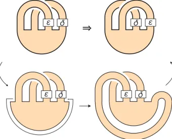
Lemma 2.3 [Outer band slide], [Invertibility]

(3) For any signs ∊ and δ, it holds that

k^∊^,δ(a, b) ＝ ℓ^δ,^∊(b,−a) ＝ k^∊^,δ(−a,−b) ＝ ℓ^δ,^∊(−b, a).

Thus these knots are invertible: −k^∊^,δ(a, b)＝k^∊^,δ(a, b), and −ℓ^∊^,δ(a, b)＝ℓ^∊^,δ(a, b).

Proof. These isotopies of the knots are induced by that of the surfaces in Figure 4. □

Figure 4: Outer band slide and its proof

δ δ ε ε

ε δ ε δ

(4)

Corollary 2.4 of Formula (2) and (3). [Switch the pair] For any signs ∊ and δ, it holds that k^∊^,δ(a, b)＝k^δ,^∊(b, a),　　ℓ^∊^,δ(a, b)＝ℓ^δ,^∊(b, a).

In a sense, formulas above are similar to those of torus knots. Contrastingly, the next is the special formula on TypeVII, VIII knots.

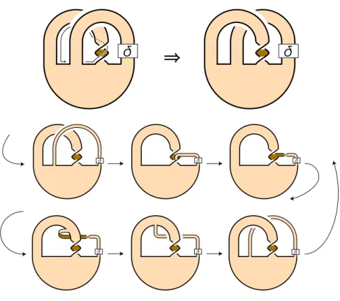
Lemma 2.5 [Inner band slide]

(4) It holds that ℓ^＋,δ(a, b)＝k^＋,δ(a−b, b), and that k^−,δ(a, b)＝ℓ^−,δ(a−b, b). Thus, ℓ^−,δ(a, b)＝k^−,δ(a＋b, b).

Proof. This isotopy of the knots is induced by that of the surfaces in Figure 5. The second formula is the mirror image of the first one by Formula (0). The third one is the inverse of the second. □

3　TypeVII knots: Case ∊＝δ.

Corollary 3.1 of Formula (3) and (4). It holds that

k^＋,＋(a, b) ＝ ℓ^＋,＋(b,−a) ＝ k^＋,＋(a＋b,−a).

The linear transformation from (a, b) to (a＋b,−a) is presented by the matrix A^＋＝

（

^{1　 1}^{−1 0}

）

. For a pair (a, b), we define

（

^a^bⁿⁿ

）

^{＝ (A}^＋

（

⁾ⁿ ^a^b

）

and call the set {(a_n, b_n)|n ∈ Z} the A^＋-orbit of (a, b). Since the matrix A^＋satisfies (A^＋)²＝

（

^{0　 1}^{−1 −1}

）

^{and (A}^＋⁾³＝−I, i.e., A^＋ is periodic of order six. This is related to the periodic monodromy of the fiber surface of the trefoil. The num- ber of the elements in the A^＋-orbit is (at most) six.

Figure 5: Inner band slide and its proof

δ δ

δ δ δ

(5)

Lemma 3.2 Among the three pairs of integers

(a, b), 　(a＋b,−a), 　(b,−a−b),

(assuming they are non-zero pairs), there exists exactly one pair is of same sign. Thus, in the A^＋-orbit of (a, b) 　(a, b),　　(a＋b,−a), 　(b,−a−b),

(−a,−b), 　 (−a−b, a), 　(−b, a＋b), there exists exactly one positive pair.

Proof. If ab > 0, then −(a＋b)a＝−ab−a²< 0, and b(−a−b)＝−ab−b² < 0. If ab < 0, then −(a＋b)a ・ b(−a−b)＝

ab(a＋b)² < 0. □

Example 3.3 Here we let k^＋(a, b) (and ℓ^＋(a, b), respectively) denote k^＋,＋(a, b) (and ℓ^＋,＋(a, b)) for short (as in [Y1]).

All 24 knots in the following table are same (isotopic) as oriented knots:

k^＋(2,−5) k^＋(−2, 5) k^＋(5,−2) k^＋(−5, 2) k^＋(−3,−2) k^＋(3, 2) k^＋(2, 3) k^＋(−2,−3) k^＋(−5, 3) k^＋(5,−3) k^＋(−3, 5) k^＋(3,−5) ℓ^＋(−5,−2) ℓ^＋(5, 2) ℓ^＋(2, 5) ℓ^＋(−2,−5) ℓ^＋(−2, 3) ℓ^＋(2,−3) ℓ^＋(−3, 2) ℓ^＋(3,−2) ℓ^＋(3, 5) ℓ^＋(−3,−5) ℓ^＋(−5,−3) ℓ^＋(5, 3) Proof of Theorem 1.1. [An algorithm to decide the required pair (a, b) in TypeVII]

First we deform the fiber surface (and the knot simultaneously) as F^∊^,δ or G^∊^,δ in Figure 1. We can assume ∊＝δ by Table 1. Then the knot is temporally presented as k^＋,＋(*, *), ℓ^＋,＋(*, *), k^−,−(*, *), or ℓ^−,−(*, *).

(Step 1) If it is k^−,−(*, *), use k^−,−(a, b)＝ℓ^−,−(b,−a) by Lemma 2.3.

(Step 2) If it is ℓ^−,−(*, *), take the mirror image ℓ^−,−(a, b)!＝k^＋,＋(a, b) by Lemma 2.2.

(Step 3) If it is ℓ^＋,＋(*, *), use ℓ^＋,＋(a, b)＝k^＋,＋(−b, a) by Corollary 3.1.

(Step 4) Find the positive pair in the A^＋-orbit of (a, b) by Lemma 3.2.

(Step 5) If it is k^＋,＋(a, b) with a > b > 0, use k^＋,＋(a, b)＝k^＋,＋(b, a) in Corollary 2.4. □

4　TypeVIII knots: Case ∊＝−δ.

Corollary 4.1 of Formula (3) and (4).

(A) It holds that

k^−,＋(a, b) ＝ ℓ^−,＋(a−b, b) ＝ k^＋,−(−b, a−b) ＝ k^−,＋(a−b,−b) ＝ k^−,＋(b−a, b).

(B) It also holds that

k^＋,−(a, b) ＝ℓ^−,＋(b,−a) ＝k^−,＋(b−a,−a)

＝　　＝　　　＝ k^＋,−(a, b) ＝ℓ^＋,−(a＋b, b) ＝k^−,＋(b,−a−b), Thus it holds that

k^−,＋(a, b)＝k^−,＋(a−b,−a＋2b).

Note that the matrix A⁻

（

＝ ^{1 −1}^−1　2

）

of the linear transformation from (a, b) to (a−b,−a＋2b) is Anosov, which is related to the monodromy of the fiber surface of the figure-eight knot.

The eigen values of A⁻ are λ＝(3＋√5)/2 and λ⁻¹＝(3−√5)/2. Their eigen vectors

(6)

x

Lv y

Lw R

⁺

R

⁻

Figure 6: Regions R^＋∪ R⁻

are v＝

（

⁻²^1＋√5

）

^{, w}^＝

（

^1−√5⁻²

）

, respectively. For a pair (a, b), we study the A⁻-orbit {(a_n, b_n)|n ∈ Z} of (a, b) with

（

^a^bⁿⁿ

）

^{＝ (A}⁻

（

⁾ⁿ ^a^b

）

^.

In the xy-plane R², we define two regions R^＋, R⁻ as

R^＋＝{(x, y)| 0 < x < y or y < x < 0}, R⁻＝{(x, y)|− x < y < 0 or 0 < x < y},

see Figure 6. The region R^＋ is essentially bounded by the line y＝x and y-axis, and R⁻ is bounded by the x-axis and the line y＝−x.

Lemma 4.2 In the A⁻-orbit of a given coprime pair (a, b), there exists exactly one pair that belongs to R^＋∪ R⁻, i.e.,

∃!n ∈ Z such that (an, bn) ∈ R^＋∪ R⁻ .

Proof. This lemma follows mainly from the characterization of Anosov matrix. In the xy-plane, the images (A⁻)ⁱ(R^＋) and (A⁻)ⁱ(R⁻) of the regions R^＋ and R⁻ by (A⁻)ⁱ (i times repeat of the linear transformation A⁻) are mutually disjoint.

Their union covers almost all R², see Figure 6:

∪

^(A⁻⁾ⁱ^(R^＋^{∪ R}⁻^)＝^R²\(Lv ∪ Lw),

i∈Z　　　　　　　

where Lv (and Lw, respectively) means the line generated by the eigen vector v (and w). Find m satisfying (a, b) ∈ (A⁻)^m (R^＋∪ R⁻), then (a_−m, b_−m) ∈ (R^＋∪ R⁻). □

Example 4.3 Here we let k⁻(a, b) denote k^−,＋(a, b), for short (as in [Y1]). All knots in the following table are same (isotopic) as oriented knots:

・・・＝k⁻(41, 26) ＝k⁻(15, 11) ＝k⁻(4, 7) ＝k⁻(−3, 10) ＝k⁻(−13, 23)＝・・・

　　　＝　　　　　　　,

・・・＝k⁻(36, 25) ＝k⁻(13, 10) ＝k⁻(3, 7) ＝k⁻(−4, 11) ＝k⁻(−15, 26)＝・・・

where, in each row, the pairs are in the A⁻-orbit.

Lemma 4.4 It holds that

k^−,＋(a, b)! ＝ ℓ^−,＋(−b,−a) ＝ k^＋,−(a,−b) ＝ k^−,＋(−b, a).

Proof. It follows from Formula (0), Lemma 2.3, and Corollary 2.4. □

(7)

Proof of Theorem 1.3. [An algorithm to decide the required pair (a, b) in TypeVIII]

First we deform the fiber surface (and the knot simultaneously) as F^∊^,δ or G^∊^,δ in Figure 1.

We have ∊＝−δ by Table 1. Then the knot is temporally presented as k^−,＋(*, *), ℓ^−,＋(*, *), k^＋,−(*, *), or ℓ^＋,−(*, *).

(Step 1) If it is ℓ^±,∓(*, *), use ℓ^±,∓(a, b) ＝k^∓,±(b,−a) in Lemma 2.3.

(Step 2) If it is k^＋,−(*, *), use k^＋,−(a, b) ＝k^−,＋(b, a) in Corollary 2.4.

(Step 3) Find the unique pair in R^＋∪ R⁻ in the A⁻-orbit of (a, b) by Lemma 4.2.

(Step 4) If the pair is in R⁻, take the mirror image k^−,＋(a, b)!＝k^−,＋(−b, a) by Lemma 4.4.

(Step 5) If (a, b) is a negative pair, use k^−,＋(a, b) ＝k^−,＋(−a,−b) in Lemma 2.2.

(Step 6) If (a, b) is in 0 < a < b but b < 2a, use k^−,＋(a, b) ＝k^−,＋(b−a, b) in Corollary 4.1(A). □

Acknowledgement. The author thanks to Dr. Toshio Saito for the information ([S]) of the potential of research interest on TypeVII, VIII knots, and for his helpful suggestion. The author also thanks to the referee for the kind advices.

References

[Ba] K L Baker, Knots on Once-punctured torus fibers, Ph. D. dissertation, The University of Texas at Austin (2004).

[Ba2] K L Baker, Surgery descriptions and volumes of Berge knots I: Large volume Berge knots, J. Knot Theory Ramifications 17 (2008), no. 9, 1077−1197.

[Bg] J Berge, Some knots with surgeries yielding lens spaces, (Unpublished manuscript, 1990).

[S] T Saito, A note on lens space surgeries: orders of fundamental groups versus Seifert genera, arXiv:math.GT/09072554.

[Y1] Y Yamada, Berge’s knots in the fiber surfaces of genus one, lens spaces and framed links, J. Knot Theory Ramifications 14 (2005), no.2, 177−188.

[Y2] Y Yamada, A family of knots yielding graph manifolds by Dehn surgery, Michigan Math. J. 53(3) (2005), 683−690.

[Y3] Y Yamada, Lens space surgeries as A’Campo’s divide knots, Algebraic & Geometric Topology 9 (2009), 397−428.