INVITED PAPER
Special Section on Recent Advances in Machine Learning for Spoken Language ProcessingSensitivity-Characterised Activity Neurogram (SCAN) for
Visualising and Understanding the Inner Workings of Deep Neural Network
Khe Chai SIM†∗a),Nonmember
SUMMARY Deep Neural Network (DNN) is a powerful machine learning model that has been successfully applied to a wide range of pat- tern classification tasks. Due to the great ability of the DNNs in learn- ing complex mapping functions, it has been possible to train and deploy DNNs pretty much as ablack boxwithout the need to have an in-depth understanding of the inner workings of the model. However, this often leads to solutions and systems that achieve great performance, but offer very little in terms of how and why they work. This paper introduces Sensitivity-characterised Activity Neorogram (SCAN), a novel approach for understanding the inner workings of a DNN by analysing and visualis- ing the sensitivity patterns of the neuron activities. SCAN constructs a low- dimensionalvisualisation spacefor the neurons so that the neuron activities can be visualised in a meaningful and interpretable way. The embedding of the neurons within this visualisation space can be used to compare the neurons, both within the same DNN and across different DNNs trained for the same task. This paper will present the observations from using SCAN to analyse DNN acoustic models for automatic speech recognition.
key words: deep neural network, visualisation, interpretability
1. Introduction
It is fascinating to see how Deep Neural Networks (DNNs) have significantly changed the way classification problems are being approached in the recent years. Its success in ad- dressing many practical real-world complex problems is cer- tainly an impactful accomplishment that has opened up the possibility for further innovations. We have been blessed with the convenience of using the DNNs as a black box, much to the liberation of letting the network learn to do the
‘right things’ as much as possible. From the engineering perspective, it is certainly nice to be able to buildend-to-end systems[1], without having to worry too much about the de- tails of the inner workings of the networks. Nevertheless, it is also equally important, for the benefit of scientific discov- ery and advancement, to study and understand the how and why behind the success of the DNNs.
Many of the existing attempts to understand the DNNs come from the vision community[2]–[5], which is not sur- prising given the nature of the task. There has not been much work from the speech community in analysing and un-
Manuscript received January 27, 2016.
Manuscript revised May 24, 2016.
Manuscript publicized July 19, 2016.
†The author was with the National University of Singapore, Singapore.
∗Presently, with Google Inc., USA.
a) E-mail: [email protected] DOI: 10.1587/transinf.2016SLI0001
derstanding the DNN acoustic models. The work in[6]at- tempts to visualise how the speech features have been trans- formed by each hidden layer in a 2-dimensional space using t-distribution Stochastic Neighbour Embedding (t-SNE)[7].
t-SNE has also been used to visualise the outputs of multi- lingual bottleneck layers[8], More recently, Nagamineet al.
investigated how DNN form phonetic categories in[9].
This paper introduces Sensitivity-characterised Activ- ity Neorogram (SCAN), a novel approach for understand- ing the inner workings of the DNNs. SCAN is based on the earlier work presented in [10], which attempts to find out
“which part of the network is doing what.” SCAN works by projecting the hidden unit activities onto a 2-dimensional space for easy visualisation and interpretation, much like the same way brain imaging techniques, such as Magnetic Res- onance Imaging (MRI)[11], are used to study human brain activities. SCAN uses anactivity vectorto characterise each neuron in the network, in terms of its sensitivity (or selec- tivity) to the different classes that the network is trained to distinguish. Moreover, the activity vectors can also be com- puted with respect to other attributes of interest. The result- ing solution involves constructing a low-dimensionalvisual- isation space, in which neurons are placed such that neurons with similar functionality (those that exhibit similar activity patterns) are close to one another. Consequently, meaning- ful regions can be conveniently identified to yield an intu- itive and interpretable visualisation of the DNNs.
SCAN is developed as a technique to assist with the analysis and interpretation of the hidden unit activity pat- terns of the DNNs. In this paper, SCAN will be used to analyse DNN acoustic models that are trained to performed Automatic Speech Recognition (ASR). DNN has been used to improve acoustic modelling in several ways. In a hybrid DNN/HMM system[12],[13], a DNN is used to predict the posterior probability of the senones, replacing the Gaussian Mixture Model (GMM) in the conventional GMM/HMM systems. DNNs have also been used to extract features such as bottleneck features[14],[15]and in building tandem ASR systems[16],[17]. There have been a number of techniques proposed to improve the robustness of DNN-based acoustic models in terms of speaker adaptation[18]–[23]and noise compensation[24]–[26].
The remainder of this paper is organised as follows.
Section 2 describes the DNN acoustic model used for the SCAN analyses in this paper. Section 3 introduces the sen- Copyright c2016 The Institute of Electronics, Information and Communication Engineers
sitivity measures and shows how these measures can be used to better understand the inner workings of DNNs. Sec- tion 4 introduces the proposed SCAN method for visualising DNNs. Section 4.3 presents the experimental findings from the various SCAN analyses. Section 5 gives a brief discus- sion and Sect. 6 concludes the paper.
2. DNN Acoustic Modelling for ASR
This section will describe the DNN acoustic model used for the analysis work presented in this paper. The DNN acoustic model is trained using the multi-condition data from the Au- rora 4 dataset[27]. There are 15.11 hours of speech (7137 utterances) in the multi-condition training set and 8.94 hours of speech (4620 utterances) in the development set. There are 7 types of noise conditions (including the clean condi- tion) and 2 channel conditions.
The input features are given by splicing 11 frames of the Linear Discriminant Analysis (LDA)[28] features.
Each LDA feature is a 40-dimensional vector projected from 39×7 Mel Frequency Cepstral Coefficients (MFCCs)[29]
features (including energy, delta and delta-delta over a 7- frame window). The DNN model has a 440-dimensional input layer and 7 hidden layers of 2048 dimension each.
The sigmoid activation function is used for all the hidden units. The output units of this network correspond to 2031 senones. This model achieved 12.5% word error rates on the Aurora 4 test set. All the acoustic models are trained using Kaldi[30]. The 40 context-independent phones are used as attributes for sensitivity measure and SCAN analyses.
3. Measuring Sensitivity
To understand the inner workings of DNNs, it is important to study the activations of the hidden units. One way of doing so is to examine the sensitivityof the hidden units with respect to some attributes of interest, such as the phone classes that the DNN is trained to classify. A hidden unit is deemed to besensitiveto a specific phone class if it has a higher probability of beingactivewhen an acoustic feature that belongs to that phone class is being fed to the network.
3.1 Sensitivity Measures
Leth(l)i (t) be the activation of hidden unitiin layerlat timet.
The sensitivity for each hidden unit with respect to attribute scan be measured as follows:
a(l)i (s)=
tγs(t)h(l)i (t)
S
s=1
tγs(t)h(l)i (t) (1)
whereγs(t) is the probability of associating attributeswith the acoustic feature at timetandS is the total number of at- tributes. For example, to measure the sensitivity of the hid- den units with respect to the phone classes,γs(t) can be ob- tained using a forward-backward algorithm (soft alignment) or a Viterbi algorithm (hard alignment). In this paper, the
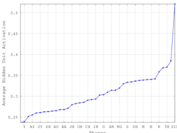
Fig. 1 Average activation of all the hidden units with respect to different phones (sorted in ascending order). For clarity, only every other phone labels are shown on the horizontal axis.
same hard alignments used to train the DNN are used com- pute the sensitivity measures. Note that
sa(l)i (s) =1 and a(l)i (s)≥0 for all s†. Therefore,a(l)i (s) effectively measures the weightage of the hidden unit’s activations with respec- tive to attribute s. A higher value of a(l)i (s) indicates that the hidden unit is expected to have a higher value of activa- tion when the acoustic frame belongs to attributes, andvice versa.
Sensitivity can also be measured for each hidden layer or the network as a whole. The sensitivity for each layer with respect to attribute scan be measured as the average sensitivity measure of each hidden unit within that layer, as given below:
˜
a(l)(s)= 1 Nl
Nl
i=1
a(l)i (s) (2)
whereNlis the number of hidden units in layerl. Likewise, the sensitivity of the network as a whole with respect to at- tributescan be measured as the avenge sensitivity of each hidden layer, as given below:
¯ a(s)= 1
L
L
i=1
˜
a(l)(s) (3)
whereLis the number of layers in the network.
Figure 1 shows the average activation of all the hid- den units with respect to different phones, ¯a(s), for all the context-independent phones, s, sorted in ascending order.
From the figure, it is clear that the network responds differ- ently to various phone classes. Some phones require more hidden units to be active than the others to achieve a good classification performance. It is particularly interesting to note that the network has a much higher average activation with respect to silence (/SIL/). This suggests that the net- work devotes many of its hidden units to the classification
†This is true for sigmoid units whereh(l)i (t) ≥ 0. For other activation functions, it may be necessary to rescale the activation values.
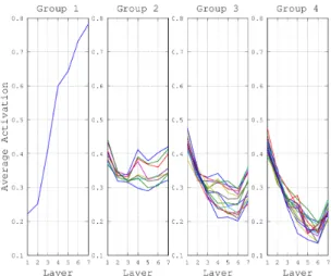
Fig. 2 Plots of average activation versus layer for four groups of phones.
Table 1 Phone groups based on the trend of average activation across different hidden layers.
Group Phones
1 SIL
2 P, F, TH, N, K, M, V, NG, B 3 T, DH, D, S, Z, HH, AH, W, ER, OW, UW, IH, G, R, UH 4 L, CH, AA, AE, AO, IY, AW,
EH, SH, JH, OY, AY, Y, ZH, EY
of silence. This is not surprising given that, in a multi-style data, the silence frames correspond to a variety of noise and channel conditions. Besides, there are relatively more silence frames in the training data compared to the other phones.
If we look at the average activations for different lay- ers, as depicted in Fig. 2, the trend can be divided into 4 groups. The grouping of the phone classes are summarised in Table 1. Group 1 consists of only theSILphone, which shows a very distinct trend compared to the rest. The net- work respond to silence with a low average activation in the first layer and this quickly increases with deeper lay- ers. The second group of phones consists of stops, frica- tives and nasals. These phones require roughly the same average activations across all the layers. This indicates that the network is steadily improving its ability to classify these phones from one layer to another. Group 3 and 4 have a de- creasing trend where more activities take place in the earlier layers, with Group 4 having a sharper decrease. This sug- gests that the network is able to classify the phones in these groups, which are mostly vowels, at a much earlier stage.
This may be explained by the fact that vowels are much easier to recognise in noisy conditions due to their stable temporal structures. By contrast, stops, fricatives and nasals are much more susceptible to distortion caused by noise. In summary, the above analyses show that the network learns to classify vowels at the earlier layers, followed by stops, fricatives and nasals, and finally concentrates most of its ef- fort in recognising silence and other background noise.
3.2 Activity Distribution Profile
To gain a better insight on how the hidden units in a network respond to different phone classes, Activation Distribution Profile (ADP) is introduced to provide a convenient way of visualising the distribution of the hidden unit activations in each layer. An ADP with respect to an attribute sis a 2- dimensional plot of the values of the following matrix:
ADPs=sort
⎛⎜⎜⎜⎜⎜
⎜⎜⎜⎜⎜
⎜⎜⎜⎜⎜
⎜⎜⎝
⎡⎢⎢⎢⎢⎢
⎢⎢⎢⎢⎢
⎢⎢⎢⎢⎢
⎢⎢⎣
a(1)1 (s) a(2)1 (s) . . . a(L)1 (s) a(1)2 (s) a(2)2 (s) . . . a(L)2 (s)
... ... ... ...
a(1)N1(s) a(2)N2(s) . . . a(L)NL(s)
⎤⎥⎥⎥⎥⎥
⎥⎥⎥⎥⎥
⎥⎥⎥⎥⎥
⎥⎥⎦
⎞⎟⎟⎟⎟⎟
⎟⎟⎟⎟⎟
⎟⎟⎟⎟⎟
⎟⎟⎠
wheresort(·) sorts a matrix column-wise in ascending or- der. Each column of the matrix corresponds to a hidden layer and each row corresponds to a hidden unit. Therefore, each column ofADPsshows the sorted distribution profile of the hidden units in each layer. It is easy to see from the ADP plots the proportion of the hidden units being active in each layer given a particular attribute.
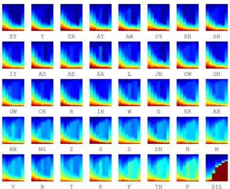
Figure 3 shows the ADP plots with respect to differ- ent phone classes. It is obvious to see that the/SIL/phone stands out as having a very distinct ADP plot compared to the other phones. There is a large number of hidden units responding actively to silence, with more hidden units in the deeper layers. Stops, such as/T/,/K/and/P/as well as nasals, such as/N/and/M/have a majority of the hidden units being moderately active (light blue), with only a rel- atively smaller number of very active hidden units. On the other hand, vowels have more active hidden units in the first hidden layer and many of the hidden units in the deeper lay- ers are not active (dark blue).
3.3 Activity Vector and Entropy Measure
Anactivity vectorcan be used to summarise the Sensitivity- characteristic of each hidden unit with respect to all the at- tributes. The activity vector for hidden unit iin layerl is given by:
a(l)i =
a(l)i (1) a(l)i (2) . . . a(l)i (S)
(4) This activity vector quantifies the function of each hidden unit. If the hidden unit is highly sensitive to a particular attribute, all except one of the elements of its activity vec- tor will be close to zero. Similarly, hidden units which re- spond to many phone classes will have larger values in the respective elements. Therefore, given thata(l)i is a probabil- ity (sum-to-one) vector, the sensitivity of each hidden unit to any attribute in general can be easily measured by com- puting the normalised entropy:
E(l)i =−
sa(l)i (s) loga(l)i (s)
−
s 1 S logS1
whereE(l)i is between 0 and 1. A lower entropy value means
Fig. 3 Plots of Activation Distribution Profile (ADP) for different phones using the rainbow colour map. Red indicates a high value and blue indicates a low value.
Fig. 4 Plots of normalised entropies for hidden units in different hidden layers. Hidden units are ordered according to ascending entropy values.
Fig. 5 Diagram showing the architecture of the DNN model after the hidden units are progressively pruned away based on the entropy measure.
Input layers are at the bottom and output layers are at the top.
higher information content, which indicates a higher sensi- tivity to a given attribute. A hidden unit is insensitive to an attribute whenE(l)i =1. This happens whena(l)i is a uniform vector,i.e. a(l)i (s)=1/S.
Figure 4 shows the entropy profile for different hidden layers of the DNN acoustic model with respect to the phone classes. The horizontal axis corresponds to the 1024 hidden units in each layer, which are sorted in ascending order ac- cording to the entropy values. The vertical axis shows the normalised entropy value for each hidden unit. There is a notable increase in the number ofinsensitivehidden units
‘plateaued’ at the top of the graph, where the normalised entropy is 1. This is clearly observed starting from layer 3,
Fig. 6 Plot of frame accuracies at different levels of pruning on the trainanddevsets.
suggesting that these hidden units do not contribute much to the final classification performance. In[10], it was found theseinsensitivehidden units can be removed from the DNN without severely affecting the classification performance.
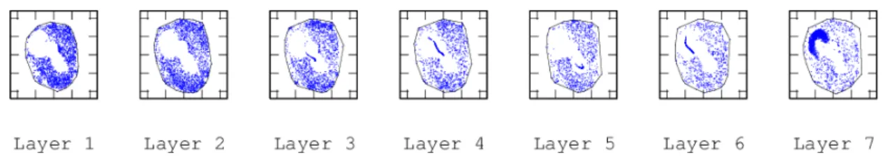
Figure 5 shows the resulting architectures of the DNN af- ter pruning away some of these hidden units according to their entropy values. The left most architecture corresponds to the case where 10% of the hidden units with the highest normalised entropy values are removed. Moving from left to right, each subsequent architecture corresponds to having an additional 10% of the hidden units removed. The rightmost architecture has 90% of the hidden units removed. From the figure, many of the hidden units being pruned away initially come from hidden layer 5. As the network is being pruned more aggressively, many hidden units from hidden layers 6 and 7 are also removed.
Figure 6 shows that the DNN can be compressed up to 60% of its original number of hidden units without severely compromising the frame accuracy performance. As reported in[31], after retraining the pruned model, it is possible to remove up to 60% of the hidden units without a significant performance degradation.
4. Sensitivity-Characterised Activity Neurogram (SCAN)
In the previous section, we described how the activity of the hidden units in the network can be analysed by measuring their sensitivity with respect to different attributes. This sec- tion will present the Sensitivity-characterised Activity Neu- rogram (SCAN) method for visualising and interpreting the activity vector of all the hidden units in a network. In the following, we will describe the workflow for creating the vi- sualisation space and how interpretable regions can be con- structed within this space.
4.1 Visualisation Space
SCAN is a visualisation method that positions the hidden units in a network on a 2-dimensionalvisualisation space such that the hidden units form clusters according to their sensitivity profiles. Hidden units that correspond to the same attributes are placed closer to one another in this visualisa- tion space. The hidden units are positioned such that those that exhibit similar sensitivity measures are placed closer together. Therefore, the visualisation space is specific to an attribute, which needs to be estimated given some speech data.
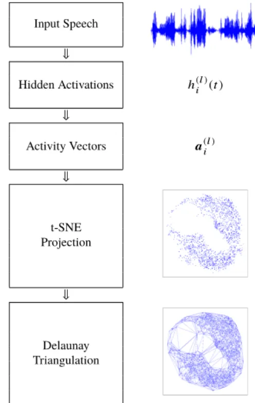
The workflow for constructing the visualisation space is illustrated in Fig. 7. To construct a visualisation space for a DNN, the first step is to compute the hidden unit ac- tivations,h(l)i (t), of all the hidden units given a set of input features. The corresponding alignments,γs(t), that maps the each acoustic feature at timetto attribute sare computed.
Next, the activity vectors, a(l)i , are computed based on the sensitivity measure using Eq. 1. Given theseactivity vectors, the location of the hidden units in thevisualisation spacecan be obtained by applying the Student’s t-distribution Stochas- tic Neighbour Embedding (t-SNE) projection method[7]or other dimensionality reduction methods. Finally, the hid- den units in the visualisation space are connected to form a triangle mesh using Delaunay triangulation[32], The trian- gle mesh is useful for colouring the visualisation space as described in Sect. 4.3.
Figure 8 depicts the condensed plot of the hidden units from all the layers of the DNN in the 2-dimensional visu- alisation space. Each hidden unit is denoted by a circle filled with colours that reflect the entropy value of that hid- den unit. A darker colour corresponds to a lower entropy, which indicates a more sensitive hidden unit. In general, the more sensitive hidden units are mostly projected onto the outer region of the space; while the less sensitive ones concentrate in the middle. This is due to the fact that the
Fig. 7 The workflow for constructing the SCAN visualisation space.
Fig. 8 Hidden units shown as circles filled with grayscale colours corre- sponding to their entropy values with respect to the phones.
t-SNE projection attempts to place the highly sensitive hid- den units (whose activity vectors are essentially close to a
‘one-hot’ vector) as far apart as possible from each other as well as from the insensitive hidden units. Consequently, these highly sensitive hidden units tend to be pushed to the edge of the space, forming the ‘extreme’ points of the con- vex hull. Less sensitive units are found in the inner region of the space. The formation of the ‘hollow’ regions is the re- sult of the gap created between the sensitive and insensitive hidden units. The strips of hidden units within the ‘hollow region’ are in fact the insensitive hidden units that form the plateauof the entropy profile graphs in Fig. 4.
4.2 Interpretable Activity Regions
Since the position of the hidden units are such that units
Fig. 10 Projection of hidden units onto thevisualisation spacewith respect to the phone classes.
Fig. 9 Interpretable regions of the visualisation space with respect to the phone classes. Some labels are omitted for clarity.
with similar sensitivity behaviour are placed closer together, it is possible to partition the visualisation space into mean- ingful and interpretable regions according to the attribute of interest. Figure 9 illustrates the interpretable phone regions in the visaulisation space. The detailed procedure for cre- ating these interpretable regions are given in [10]. From the figure, it is clear that the hidden units (from all the lay- ers) form clear phone-dependent regions in the visualisation space. For example, the top left region corresponds to si- lence. Besides, regions that belong to similar phones, such as/EH/and/AY/, are found next to each other. The size of the regions roughly corresponds to the number of hidden units that are sensitive to the corresponding phones. Phones with a larger region may be more difficult to classify and therefore require more hidden units.
Figure 10 shows the projection of the hidden units for the different layers of the DNN model in thevisualisation space. A common visualisation space is constructed for all the hidden units across different layers so that they can be easily compared and interpreted. In fact, as shown in[10], it is possible to compare hidden units from different DNNs as long as the same sensitivity measure is used to characterise all the hidden units. There are several interesting observa- tions that can be made from Fig. 10. The shape of the visu- alisation space is given by the convex hull of the projection of the hidden units in this space. In general, the shape of the visualisation spaces are rather similar across different hid- den layers. The distribution of the hidden units varies con- siderably across different hidden layers. This suggests that the functionality of the hidden units changes from one hid- den layer to another. The hidden units of the first layer are rather uniformly distributed over the entire space except the
‘hollow’ region at the top left and the middle of the space.
Fig. 11 Examples of SCAN plots for phones/SIL/,/V/,/P/, and/EY/
(left to right).
In layer 3, there is a region with a higher concentration of hidden units at the top. According to Fig. 9, this region cor- responds to the/TH/phone, which according to Table 1 and Fig 3, have a relatively higher average activations in the mid- dle layers.
4.3 Visualisation Using SCAN
With the interpretable visualisation space, it is possible to easily visualise the activity patterns of the hidden units.
Each triangle in the Delaunay triangle mesh is coloured with a linear gradient colour obtained by interpolating the colour of the vertices. Since each vertex corresponds to one hid- den unit, the vertex colour is chosen to reflect the activation value of that hidden unit. In the following examples, the activation values are indicated by the brightness of the red colour.
Figure 11 shows four example plots from visualising the hidden unit activations using SCAN. The left-most plot shows the SCAN visualisation of a silence (/SIL/) frame, where the active hidden units are mostly concentrated at the top left corner of the visualisation space. This is expected as the hidden unit in this region has a higher probability of being active for silence, as depicted in Fig. 9. The sec- ond plot from the left corresponds to the phone /V/, with active hidden units concentrated in the top region. This is again consistent with the interpretable regions as shown in Fig. 9. Similarly, the last two plots are for the/P/and/EY/
phones, where visible active clusters can be observed in the top-right and bottom-left regions, respectively.
SCAN can also be used to visualise in realtime the evolution of the activation patterns frame by frame. This allows the temporal changes in the activity patterns to be monitored. Figure 12 shows an example of visualising the evolution of the hidden unit activations from silence/SIL/
to/AA/. The plots clearly show the transition of the active region from top left to bottom right.
5. Discussions
So far, we have described SCAN as a way of organising
Fig. 12 Examples of SCAN plots showing the evolution of the activation pattern from/SIL/to/AA/
at 50 milliseconds intervals (left to right).
Fig. 13 Hidden layer activation: unstimulated (left) and stimulated (right).
Fig. 14 Phone-specific stimulation points for stimulated deep learning.
the hidden units in a 2-dimensional visualisation space, so that active hidden units tend to be close to one another.
This shows that the activation patterns of the hidden units are somewhat correlated. This also explains why the affine transformation matrix in the hidden layers can be approxi- mated using low-rank approximations[33]–[35]. In the low- dimensional visualisation space, SCAN also establishes re- lationships between the hidden units. Through Delaunay triangulation[32], hidden units are connected to form a tri- angle mesh in the visualisation space. These connections identify the neighbours for each hidden unit, which can be used as regularisation when training or adapting the DNNs.
Stimulated Deep Learning (SDL)[36] is another re- lated approach that explicitly constrains the hidden unit ac- tivations to form visualisable and interpretable regions. Un- like SCAN, SDL lays out the hidden unit of each hidden layer in a simple grid and applies constraints during training to control the activation pattern of the hidden units. Fig- ure 13 shows the activation patterns of two networks, the left one corresponds to a standard (unstimulated) DNN and the right one corresponds to a stimulated DNN. The lat- ter shows a clear structured activation pattern as a result of SDL. Phone-specific stimulation points (see Fig. 14) are ap- plied to different positions in the grid such that the hidden units that are closer to the stimulation points tend to be more sensitive to the corresponding phones. It was found in[36]
that SDL also acts as a form of regularisation that improves
the recognition performance.
6. Conclusions
This paper has presented Sensitivity-characterised Activity Neurogram (SCAN), a novel technique for visualising and understanding DNN in terms of the sensitivity patterns of its hidden units towards some attributes of interest. SCAN is used to analyse a DNN acoustic model trained on the multi-condition data from the Aurora 4 dataset for automatic speech recognition. By analysing the sensitivity measures of the hidden units with respect to the phone classes, it is found that there are more hidden units responding to silence, stops, fricatives and nasals as they are much harder to recognise in noisy conditions. Furthermore, by examining the entropy of these activity patterns, it is possible to identify insensitive hidden units and up to 40% of these hidden units can be re- moved from the network without severely affecting the clas- sification performance. SCAN constructs a 2-dimensional visualisation space such that hidden units that exhibit simi- lar activity patterns are placed closer together in this space.
Interpretable phone regions are constructed in this space to yield a meaningful visualisation of the hidden unit activa- tions. Some phone regions are bigger than the others, sug- gesting that these phones are more difficult to recognise and require more ‘attention’ from the DNN.
References
[1] A. Graves and N. Jaitly, “Towards end-to-end speech recognition with recurrent neural networks,” Proc. 31st International Conference on Machine Learning (ICML-14), pp.1764–1772, 2014.
[2] G.D. Garson, “Interpreting neural-network connection weights,” AI Expert, vol.6, no.4, pp.46–51, April 1991.
[3] K. Simonyan, A. Vedaldi, and A. Zisserman, “Deep inside convolutional networks: Visualising image classification models and saliency maps,” Computing Research Repository (CoRR), vol.abs/1312.6034, 2013.
[4] A. Mahendran and A. Vedaldi, “Understanding deep image repre- sentations by inverting them,” 2015 IEEE Conference on Computer Vision and Pattern Recognition (CVPR), pp.5188–5196, 2015.
[5] M.D. Zeiler and R. Fergus, “Visualizing and understanding con- volutional networks,” Computer Vision – ECCV 2014, vol.8689, pp.818–833, 2014.
[6] A.R. Mohamed, G. Hinton, and G. Penn, “Understanding how deep belief networks perform acoustic modelling,” Proc. ICASSP, pp.4273–4276, March 2012.
[7] L. van der Maaten and G. Hinton, “Visualizing data using t-SNE,” J.
Machine Learning Research, vol.219, no.1, pp.1–48, 2008.
[8] N.T. Vu, J. Weiner, and T. Schultz, “Investigating the learning ef- fect of multilingual bottle-neck features for ASR,” Proc. Interspeech, 2014.
[9] T. Nagamine, M.L. Seltzer, and N. Mesgarani, “Exploring how deep neural networks form phonemic categories,” Proc. Interspeech, 2015.
[10] K.C. Sim, “On constructing and analysing an interpretable brain model for the DNN based on hidden activity patterns,” Proc. Au- tomatic Speech Recognition and Understanding (ASRU), pp.22–29, 2015.
[11] A.G. Filler, “The history, development and impact of computed imaging in neurological diagnosis and neurosurgery: CT, MRI, and DTI,” Nature Precedings, vol.7, no.1, pp.1–69, 2009.
[12] G. Hinton, L. Deng, D. Yu, G. Dahl, A.-R. Mohamed, N. Jaitly, A.
Senior, V. Vanhoucke, P. Nguyen, T.N. Sainath, and B. Kingsbury,
“Deep neural networks for acoustic modeling in speech recogni- tion,” IEEE Signal Processing Magazine, vol.29, no.6, pp.82–97, Nov. 2012.
[13] G.E. Dahl, D. Yu, L. Deng, and A. Acero, “Context-dependent pre–
trained deep neural networks for large-vocabulary speech recogni- tion,” IEEE Trans. Audio, Speech, and Language Processing, vol.20, no.1, pp.30–42, Jan. 2012.
[14] J. Gehring, Y. Miao, F. Metze, and A. Waibel, “Extracting deep bottleneck features using stacked auto-encoders,” Proc. ICASSP, pp.3377–3381, May 2013.
[15] D. Yu and M. Seltzer, “Improved bottleneck features using pre- trained deep neural networks,” Proc. Interspeech, pp.237–240, Aug.
2011.
[16] M. Ferras and H. Bourlard, “MLP-based factor analysis for tandem speech recognition,” Proc ICASSP, pp.6719–6723, May 2013.
[17] S.P. Rath, K.M. Knill, A. Ragni, and M.J.F. Gales, “Combining tandem and hybrid systems for improved speech recognition and keyword spotting on low resource languages,” Proc. Interspeech, pp.835–839, Sept. 2014.
[18] F. Seide, G. Li, X. Chen, and D. Yu, “Feature engineering in con- text-dependent deep neural networks for conversational speech tran- scription,” Proc. ASRU, pp.24–29, Dec. 2011.
[19] G. Saon, H. Soltau, D. Nahamoo, and M. Picheny, “Speaker adap- tation of neural network acoustic models using i-vectors,” Proc.
ASRU, pp.55–59, Dec. 2013.
[20] O. Abdel-Hamid and H. Jiang, “Fast speaker adaptation of hybrid NN/HMM model for speech recognition based on discriminative learning of speaker code,” Proc. ICASSP, pp.7942–7946, May 2013.
[21] A. Senior and I. Lopez-Moreno, “Improving DNN speaker indepen- dence with i-vector inputs,” Proc. ICASSP, pp.225–229, May 2014.
[22] Y. Miao, H. Zhang, and F. Metze, “Towards speaker adaptive train- ing of deep neural network acoustic models,” Proc. Interspeech, pp.2189–2193, Sept. 2014.
[23] P. Swietojanski and S. Renals, “Learning hidden unit contribu- tions for unsupervised speaker adaptation of neural network acoustic models,” Proc. SLT, pp.171–176, Dec. 2014.
[24] M.L. Seltzer, D. Yu, and Y. Wang, “An investigation of deep neu- ral networks for noise robust speech recognition,” Proc. ICASSP, pp.7398–7402, May 2013.
[25] B. Li and K.C. Sim, “Noise adaptive front-end normalisation based on vector Taylor series for deep neural networks in robust speech recognition,” Proc. ICASSP, pp.7408–7412, May 2013.
[26] B. Li and K.C. Sim, “A spectral masking approach to noise-ro- bust speech recognition using deep neural networks,” IEEE/ACM Trans. Audio, Speech and Language Processing, vol.22, no.8, pp.1296–1305, Aug. 2014.
[27] G. Hirsch, “Experimental framework for the performance evaluation of speech recognition front-ends on a large vocabulary task, version 2.0,” ETSI STQ-Aurora DSR Working Group, 2002.
[28] G. Saon, M. Padmanabhan, R. Gopinath, and S. Chen, “Max- imum likelihood discriminant feature spaces,” Proc. ICASSP, pp.II1129–II1132, 2000.
[29] S.B. Davis and P. Mermelstein, “Comparison of parametric repre- sentations for monosyllabic word recognition in continuously spo- ken sentences,” IEEE Transactions on Acoustic, Speech and Signal
Processing, vol.28, no.4, pp.357–366, 1980.
[30] D. Povey, A. Ghoshal, G. Boulianne, L. Burget, O. Glembek, N.
Goel, M. Hannemann, P. Motlicek, Y. Qian, P. Schwarz, J. Silovsky, G. Stemmer, and K. Vesely, “The Kaldi speech recognition toolkit,”
Proc. ASRU, pp.1–4, Dec. 2011.
[31] K.C. Sim and G. Mantena, “A comparison of model parameter reduction methods for deep neural networks,” Proc. 1st Machine Learning in Spoken Language Processing (MLSLP), 2015.
[32] D.T. Lee and B.J. Schachter, “Two algorithms for constructing a De- launay triangulation,” International Journal of Computer and Infor- mation Sciences, vol.9, no.3, pp.219–242, June 1980.
[33] D. Yu, F. Seide, G. Li, and L. Deng, “Exploiting sparseness in deep neural networks for large vocabulary speech recognition,” Proc.
ICASSP, pp.4409–4412, March 2012.
[34] J. Xue, J. Li, and Y. Gong, “Restructuring of deep neural network acoustic models with singular value decomposition,” Proc. Inter- speech, pp.2365–2369, Aug. 2013.
[35] T.N. Sainath, B. Kingsbury, V. Sindhwani, E. Arisoy, and B.
Ramabhadran, “Low-rank matrix factorization for deep neural net- work training with high-dimensional output targets,” Proc. ICASSP, pp.6655–6659, May 2013.
[36] S. Tan, K.C. Sim, and M. Gales, “Improving the interpretability of deep neural networks with stimulated learning,” Proc. Automatic Speech Recognition and Understanding (ASRU), pp.617–623, 2015.
Khe Chai Sim received the B.A. &
M.Eng. degrees in electrical and information sciences from the University of Cambridge, U.K., in 2001. He then received the M.Phil.
degree in computer speech, text and internet technology in 2002 from the same university.
He joined the Machine Intelligence Laboratory, Cambridge University Engineering Department as a research student and completed his doctoral dissertation: “Structured Precision Matrix Mod- elling for Speech Recognition” in 2006 under the supervision of Professor Mark Gales. He was an Assistant Professor at the National University of Singapore between 2008 to 2016. He is a Senior Research Scientist at Google since 2016. He has worked on the DARPA-funded EARS project from 2002-2005 and the GALE project from 2005-2006. He has also participated in various NIST evaluations: Rich Transcription (2004), Machine Translation (2006), Language Recognition (2007) and Speaker Recognition (2008). He is a recipient of the Google Faculty Research Award 2014.