1次元周期的2次元Stokes 流に対する基本解法(解析学における問題の計算機による解法)

1

次元周期的

2

次元

Stokes

流に対する基本解法

Fundamental

Solutionxs

Method for

Two-Dimensional

Stokes Flow

Problems

with

One-Periodic

Periodicity

電気通信大学情報工学科 緒方秀教(Hidenori Ogata)

Department _of Computer Science,

The University of Electro-Communications

July 5,

2007

Abstract

In thispaper, weproposeafundamental solution method for the problems of two-dimensional Stokes flow past aone-dimensional periodic array of cylinders. In the presented method, the solution is approximated by a superposition of the periodic Stokeslets, the periodic fundamental $8olutions$ of the Stokes flow equation. The numerical example included in this paper show the effectiveness of the presented method.

1

Introduction

Flow problems with spatial periodicity are attracting subjects from the

viewpoint of theoretical fluid mechanics and important in applications to

science and engineering. The aim of this paper is to present a fundamental

solution method for the problems of two-dimensional Stokes flows past a

one-dimensional periodic array of cylinders as shown in Figure 1.

There

are

many

works

on

spatially periodic flows

a.s

follows.

As a

work

on

periodic potential flows, Ogata et al. presented

a

charge

sim-ulation method (fundamental solution method) for numerical conformal

mappings of two-dimensional Euclidean domains, which is identified with

one-dimensional complex domain, _with one-dimensional periodic

periodic-ity [19] and applied their method to the analysis oftwo-dimensional

Oseen

flow, TaIIldda and$\cdot$ Fujikawa

studied

the problem of steady

two-$cli_{Il1}ellsioI\iota a1$

Oseen

flow past an infinite

row

of circular cylinders [22]. As

works $011$ periodic

Stokes

flow, the problemswith which

we

are concerned

in

this paper, Hasimoto prcsented the periodic fundamental solution method

of the two of thrce-dimcnsional Stokes flow equation and applied it to

the analysis of Stokes flow past a periodic array of spheres [7], which was

improved by Sangani and Acrivos [20]. Ishii presented the fundamental

solution of three-dimensional Stokes fiow with planar periodicity and

ap-plied it to the study of three-dimensional

Stokes

flow problem with planar

arrays of small spheres [8]. In addition,

as works on

application of periodic

Stokes flow studies, Liron presented studies of Stokes flow due to

an

infinit

array of Stokeslets, which

are

applied to the analysis of ciliary transport

[12. 13, 14].

The fundamental solution method is

a

numerical solver of partial

dif-ferential equation problems and is widely used in science and engineering,

especially. in potential problems, where the method is usually called the

“charge simulation method” $[15, 21]$, for the

reasons

that it is easy to

pro-gram, (ii) its computational cost is low and (iii) it achieves high accuracy

under some conditions. In this method, the solution

is

approximated by

a

linear

combination of

the

fundamental

solutions of the partial

differen-tiation

operator with

singularities

outside the problem domain.

In

terms

of physics, the potential which

is

the solution of

a

potential problem is

approximated by a superposition of the Coulomb potentials due to the

charges positioned outside the problem domain. Katsurada and Okamoto

showed the solvability and the high accuracy of the fundamental solution

method from theoretical viewpoints [9, 10, 11]. As works on applications

of the fundamental solution method, Amano et al. presented numerical

conformal mappings by the fundamental solution method [1, 2, 3]. Related

to this paper, Chuwang and Wu presented

a

fundamental solution method

for Stokes flow problems, whose approximation is based

on

the Stokeslet

[4].

It is, however, difficult to apply the fundamental solution method by

Cl$mwaIlg$ and Wu to

our

problem of periodic Stokes flow because the

ap-proximation of Chuwang and Wu’s method may not be able to

approxi-mate accurately the solution of

our

periodic problem which may include

tlze Stokeslet so that it illustrates the flow due to an infinite periodic

ar-ray of concentrated forces of equal magnitude and construct an

approx-imate solution by a linear combination of the above periodic Stokeslet.

It is expected that this method inherits the advantages of the ordinary

fundamental solution method and

can

approximate the solution including

periodic functions with high accuracy. We here remark that, as work

re-lated to

our

method, Ogata et al. presented fundamental solution methods

for two-dimensional potential problems with one-dimensional periodicity

[19], two-dimensional Stokes flow problems with a two-dimensional

peri-odic array of cylinders [18], three-dimensional Stokes flow problems with

a two

or

three-dimensional periodic array of obstacles $[16, 17]$

.

Greengard

and Kropinski presented an integral equation method for two-dimensional

Stokes fl$ow$ problemsin double-periodic domains, which is based on elliptic

function theory and incorporated into the fast multipole method [6]. and

Zick

and Homsy alsopresented

an

integral equation

method

for Stokes flow

problems with

a

periodic array of spheres, which is based on the periodic

fundamental solution of the Stokes flow equation [23].

The contents of this paper are as follows. In

Section

2, we formulate

mathematically our problem and prepare some notations. In Section 3, we

present a fundamental solution method for

our

problems. In Section 4, we

show a typical numerical example of our method. In Section 5,

we

givc

concluding remarks.

2

Formulation

of

Problems

We first

formulate our

problem mathematically and give

some

notations.

Throughout this paper,

we

denote by $\mathbb{Z}$ the set of all the integers and by $\mathbb{Z}$

the set of all the complex numbers. We denote the Cartesian coordinates

of the

two-dimensional

Euclidean plane $\mathbb{R}^{2}$ by

$(x_{1}, \prime x_{2})$ and identify a point

$(x_{1},x_{2})\in \mathbb{R}^{2}$ with the complex number _{$z=x_{1}+ix_{2}\in \mathbb{C}$}

.

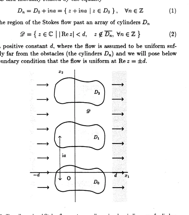
We here consider thc problem of a stationary two-dimensional Stokes

flow past a one-dimensional periodic array of cylinders

as

shown in Figure

1). In the figure, $D_{n},$ $n\in \mathbb{Z}$

are

the cylinders of the

same

shape which

are arranged in a one-periodic array of period $ia(a>0)$

.

In terms of

plaIie $\mathbb{C}$ alid rnutually related by tlie equality

$D_{n}=D_{0}+ina=\{z+ina|z\in D_{0}\}$ , $\forall n\in \mathbb{Z}$ (1)

$\overline{\swarrow}^{c_{:}}$ is the region of the Stokes flow past an array of cylinders $D_{r\iota}$

$\ovalbox{\tt\small REJECT}=\{z\in \mathbb{C}||{\rm Re} z|<d, z\not\in\overline{D_{n}}, \forall n\in \mathbb{Z}\}$ (2)

with a positive constant $d$, where the flow is assumed to be uniform

suf-ficiently far from the obstacles (the cylinders $D_{n}$) and we will pose below

the boundary condition that the flow is uniform at ${\rm Re} z=\pm d$

.

Figure1: Two-dimensional Stokes flow past a one-dimensionalperiodic arrayofcylinders.

3

Fundamental Solution

Method

Our

problem of the periodic Stokes flow is

given

in terms of

mathematics

by

equatioIi

Stokes flow equation $\mu\Delta v-\nabla p=0$ in

9

(3)

continuity equation $\nabla\cdot v=0$ in

9

(4)

boundary conditions $v=0$ on $\partial D_{n}(n\in \mathbb{Z})$ (5)

$v=(U,0)$ on $lx_{1}=\pm d$

.

(6)

From (4), there exists a stream function $\Psi(x_{1}, x_{2})$ such that it gives the

velocity $v=(v_{1}, v_{2})$ by

$v_{1}= \frac{\partial\Psi}{\partial x_{2}}$

,

$v_{2}=- \frac{\partial\Psi}{\partial x_{1}}$

.

(7)

From

(3) and (7),

we

can easily find that

$\Delta^{2}Psi=0$_, (8)

that is, the stream function $\Psi$ is a biharmonic function. Therefore, the

stream function

can

be written as

$\Psi(z)={\rm Im}\{\overline{\sim_{\wedge\prime}\sim}\varphi(z)+\int^{z}\psi(z’)dz’\}$ $(z=x_{1}+ix_{2})$ (9)

with analytic functions $\varphi(z),$ $\psi(z)$, which is called “Goursat’s

representa-$tion[5]$

.

Based

on

(9), the complex velocity

is

written

as

$\dagger l^{r}\equiv v_{1}-iv_{2}=2i\frac{\partial\tilde{\Psi}}{\partial}=\overline{z}\varphi’(z)-\overline{\varphi}(\overline{z})+\psi(z)$

.

(10)

As

a

fundamental solution of the Stokes flow equation (3) and the

conti-nuity equation (4), we know the “Stokeslet”, the flow such that the analytic

function $\varphi(z)_{:}\psi(z)$ in (9) is given by

$\varphi(z)=-Q_{0}\log(z-\zeta_{0})$, (11) $\psi(\approx)=\overline{Q_{0}}(z-\zeta_{0})\log(z-\zeta_{0})-Q_{0^{\frac{z-2{\rm Re}\zeta_{0}}{z-(0}}}$ (12)

where

$Q_{()}$

is

a

complex constant and $\zeta_{0}$ is

a

fixed point

in

the complex

plane, and the complex velocity is given by

Ill terms of physics, the

Stokeslet

is a

Stokes

flow due to a concentrated

$force-8\pi\mu Q_{0}=-8\pi\mu({\rm Re} Q_{0}, {\rm Im} Q_{0})$

on

the point$\zeta_{0}$ in the complex plane.

Therefore, in the fundamental solution method for ordinary Stokes flow

problem in a domain

9,

the analytic function $\varphi(z),$ $\psi(z)$ in (9)

are

ap-proximated by

$\varphi(z)\simeq-\sum_{j=1}^{N}Q_{j}\log(z-\zeta_{j})$, (14)

$\psi(z)\simeq\sum_{j=1}^{N}\overline{Q_{j}}(z-\zeta_{j})\{\log(z-\zeta_{j})-1\}$ , (15)

and, then, the complex velocity

is

approximated by

$W \simeq 2\sum_{j=1}^{N}\overline{Q_{j}}1og|z-\zeta_{j}|-2\sum_{j=1}^{N}Q_{j^{\frac{{\rm Re}(z-\zeta_{j})}{z-\zeta_{j}}}}$

.

(16)

In (14-16), $\zeta_{j},$ $j=1,2,$

$\ldots,$ $N$ are the singularity points given in the

exte-rior ofI and $Q_{1,}.Q_{2},$ $\ldots,Q_{N}$ are the complex coefficients to be determined

so that the flow satisfies the boundary conditions in

a

sufficient accuracy.

In terms of physics, the above approximation (14-16) illustrates the

su-perposition of the Stokes flows due to the concentrated $forces-8\pi\mu Q_{j}=$

$-8\pi\mu({\rm Re} Q_{j}, {\rm Im} Q_{j}),$ $j=1,2,$ $\ldots$ ,$N$

on

the point $\zeta_{j},$ $j=1,2,$ $\ldots$ , $N$

.

It is, however, difficult to approximate the solution of

our

problem by

the ordinary fundamental solution method (14-16) because these

approxi-mation

are

not periodicfunctions. Therefore,

we

have to modify the above

fundamental solution

method so

that it

can

approximate the periodic

so-lutions of

our

problems. A primitive IIlodification may be arranging the

Stokeslets in a periodic array, that is, approximate the analytic functions

$\varphi(z),$ $\psi(z)$ by

$\varphi(z)\simeq-\sum_{n\in \mathbb{Z}}\sum_{j=1}^{N}Q_{j}\log(z-(\zeta_{j}+ina))$

,

(17)

but the infinite sums in the above approximation are generally divergent as

tlrey are. Then, we modify the infinite

sums

so that they are convergent,

IldIIlely,

$\sum_{\prime,n\in\wedge}\sum_{jn=1}^{N}Q_{j}\log(z-(\zeta_{j}+ina))arrow\sum_{j=1}^{N}Q_{j}\{\log(z-\zeta_{j})+\sum_{n\neq 0}[\log(1-\frac{\prime\sim\prime-\zeta_{j}}{ina})+\frac{z-\zeta_{j}}{ina}]$

$= \sum_{j=1}^{N}Q_{j}$log sinh $[ \frac{\pi}{a}(z-\zeta_{j})]$

,

(19)

$\sum_{n\in Z}\sum_{j=1}^{N}Q_{j^{\frac{z-2{\rm Re}(\zeta_{j}+ina)}{\sim\prime-(\zeta_{j}+ina)}=}}.\sum_{j=1}^{N}Q_{j}(z-2{\rm Re}\zeta_{j})\sum_{n\in \mathbb{Z}}(\frac{1}{z-\zeta_{j}-ina}+\frac{1}{ina})$

$arrow\sum_{j=1}^{N}Q_{j}(z-2{\rm Re}\zeta_{j})\{\frac{1}{z}+\sum_{n\neq 0}(\frac{1}{\approx-\zeta_{j}-ina}+\frac{1}{ina})\}$

$= \frac{\pi}{a}\sum_{j=1}^{N}Q_{j}(z-2{\rm Re}$ (;)

coth

$[ \frac{\pi}{a}(z-\zeta_{j})]$

,

(20)

and we have

$\varphi(z)\simeq\varphi_{N}(z)\equiv-\sum_{j=1}^{N}Q_{j}$logsinh $[ \frac{\pi}{a}(z-\zeta_{j})]$ , (21)

$\psi(z)\simeq\psi_{N}(z)\equiv\sum_{j=1}^{N}\overline{Q_{j}}$ logsinh $[ \frac{\pi}{a}(z-\zeta_{j})]-\frac{\pi}{a}\sum_{j=1}^{N}Q_{j}(z-2{\rm Re}\zeta_{j})$coth $[ \frac{\pi}{a}(z-\zeta_{j})]$

.

(22)

These give an approximate complex velocity by

$W\simeq W_{N}\equiv u_{1}^{(N)}-iu_{2}^{(N)}$

$\equiv 2\sum_{j=1}^{N}\overline{Q_{j}}$log sinh $[ \frac{\pi}{a}(z-\zeta_{j})]|-\frac{2\pi}{a}\sum_{j=1}^{N}Q_{j}{\rm Re}(z-\zeta_{j})$coth $[ \frac{\pi}{a}(z-\zeta_{j})]$

.

(23)

The approximation (21-23) is suitable for our problem of periodic

Stokes

expected to iIlherit the advaIltages of the ordinary $fuIldaInental$ _solution

luethod that it is easy to compute and it gives approximation with high

accuracy. This approximationis given by a linear coInbination of tfie

‘Mpe-riodic Stokeslct”, the pe‘Mpe-riodic fundamental solutions of the Stokes flow

equation and the continuity equation and, in terms of physics, it

illus-trates the superpositions of the flows due to an infinite periodic array of

concentrated forces $-8\pi\mu Q_{j}=-8\pi\mu({\rm Re} Q_{j}, {\rm Im} Q_{j}),$ $j=1,2,$ $\ldots$

,

$N$

on

the

points $\zeta_{j}+ina,$ $n\in \mathbb{Z}$

.

Thecomplex coefficients $Q_{j}$

are

determined bythe collocationcondition,

the condition that the approximate velocity (23) satisfies the boundary

conditions (6) only at a finite number of boundary points. Namely,

we

choose boundary points

$(+)$ $(+)$

$z_{1}^{(0)},$$z_{2}^{(0)},$

$\ldots,$$z_{N_{0}}^{(0)}\in\partial D_{0}t-$

) $(-)$

$\approx 1$ ,$z_{2}$ ,

...,

$z_{\bigwedge_{+}^{\gamma}}^{(+)}\in\{z\in \mathbb{C}|{\rm Re} z=d\}$ , $z_{1}$ ,$z_{2}$

,

...,

$z_{N_{-}}^{(-)}\in\{z\in \mathbb{C}|{\rm Re} z=-d\}$

$(N_{0}+N_{+}+N_{-}=N)$

(24)

and

pose

the boundary

contitions

(6)

on

$M_{N}^{J’}$ at the above points

$\ddagger\phi_{N}^{t^{*}}(z_{i}^{(0)})=0$ $i=1,2,$

. .

.,

_{$N_{0}$}, (25)

$W_{N}(z_{i}^{t+)})=U$ _$i=1,2,$

$\ldots,$ $1V+$

,

(26)

$W_{N}^{r}(z_{i}^{t-)})=U$ $i=1,2,$

$\ldots,$ $N_{-}$

.

(27)

The equations (25-27) form a system of linear equations with respect to

the coefficients$Q_{1},Q_{2},$ $\ldots$ ,$Q_{N}$

.

We determinethe coefficient$sQ_{j}$ bysolving

the above system of linear equations and obtain the approximate velocity

$\iota\prime \mathfrak{s}_{N}^{r}$

.

4

Numerical

Example

We here show a numerical example of the presented $met_{1}hod$

.

All the

com-putations

were

carried out using

programs

coded in $C++with$ double

precision working.

The example is the problem of Stokes flow past

a

periodic array of

circular cylinders, that is, the Stokes flow problem in the domain

with

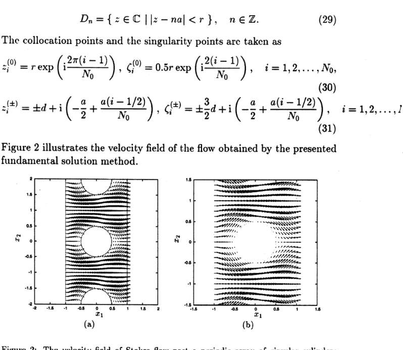
$D_{n}=\{\approx\in \mathbb{C}||z-na|<r\}$, $n\in \mathbb{Z}$

.

(29)

The collocation points and the singularity points are taken

as

$\sim\sim i(0)=\gamma$

.

exp _{$( i\frac{2\pi(i-1)}{N_{0}}),$}

$\zeta_{i}^{(0)}=0.5r\exp(i\frac{2(i-1)}{N_{0}})$

,

$i=1,2,$

$\ldots,$$N_{0}$

,

(30)

$\approx i(\pm)=\pm d+i(-\frac{a}{2}+\frac{a(i-1/2)}{\lrcorner V_{0}}),$

$\zeta_{i}^{(\pm)}=\pm\frac{3}{2}d+i(-\frac{a}{2}+\frac{a(i-1/2)}{N_{0}})(31)i=1,2,$$\ldots,$

$1$

Figure

2

_{illustrates the velocity field of tbe flow obtained by the presented}

fundamental solution

method.

Figure 2: The velocity field of Stokes flow past a periodic array

or

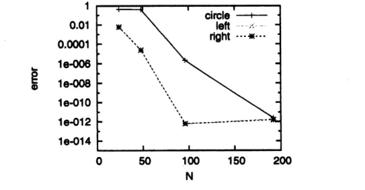
circular cylinders computed by the presented method. The figure (b) is a magnification of the figure (a).

In orderto estimate the accuracy ofthe presented method,

we

computed

tlle

error

on

the

boundaries

$\epsilon(circle)=\sup_{z\in\partial D_{0}}\frac{|W_{N}(z)|}{U}$. $\epsilon(left)=\sup_{B\epsilon z=-d}\frac{|7W_{N}(z)-U|}{U}$

,

$\epsilon(rig1_{1}t)=s\iota\iota p\frac{|fW_{N}(z)-U}{U}{\rm Re} z=d$

where the suprima

are

actuallycolnputed as the maxima

on 1000

bouIldary

points distributed by using the uniform random numbers. Figure 3 shows

the error

estimates

(32) as the totalnumbers of the nodes $N=3N_{0}$

,

though

we cannot distinguish between the

error on

the left boundary $\epsilon(left)$ and

the error

on

the right boundary $\epsilon(right)$

.

From

this figure, we find that

the

errors on

the left and right boundaries $\epsilon(left),$ $\epsilon(right)$

are

of the order of

the square of the

error on

the surfaces of the cylinders $\epsilon(circle)$ with the

same number

of the nodes, and the total

error

decays exponentially

as

the

number of nodes $N=3_{1}V_{0}$

increases.

$\dot{\Phi\xi}$

$0$ 50 100 150 200 $N$

Figure 3: The error $e8timate8$ ofthe presented method as functions of the total number

of the nodes $N=3N_{0}$

.

5

Concluding

Remarks

In this paper, we presented the fundamental solution method for the

prob-lems of two-dimensional Stokes flow past a one-dimensional periodic array

of cylinders. We obtained

our

method by using the biharmonic function

theory based

on

analyticfunctions and by modifying the Stokeslet included

in the approximation so that the method gives a good approxiInation of

$tl\iota e$ solution including periodic

functions.

The

numerical

exaInples

for a

problem with

circular cylinders shows an

exponential

convergence

of

our

Acknowledgement

This work is supported bya Grant-in-Aidfor Scientific Research (C) (No.18560054),

Japan Society for

Promotion

of

Science.

References

[1] K. Amano, A charge simulation method for the numerical conformal

mapping

of interior,

exterior

and doubly-connected domains,

J.

Com-put. Appl. Math.

53

(1994)

_353-370.

[2] K. Amano, _{A charge simulation method for numerical conformal}

map-ping

onto circular and radial slit domains,

_SIAM

_J.

_Sci.

_{Comput. 19}

(1998)

_1169-1187.

[3] _{K. Amano, D.} Okano, H. Ogataand M. Sugihara, Numerical conformal

mappings of unbounded multiply-connected domains by the charge

simulatioll method, Bull. Malaysian Math.

Sci. Soc.

26 (2003)

3551.

[4]

A.T. Chuwang

and

T.Y.-T.

Wu, Hydrodynamics of

low-Reynolds-number flow. Part 2. Singularity method for Stokes flow, J. Fluid

Mech.

67

(1975) $78\overline{/’}-815$

.

[5]

\’E.

Goursat, Sur l’\’equation $\Delta\Delta u=0$

,

Bull. Soc. Math. France 26

(1898)

_236-237.

[6] L. Greengard and M.C. Kropinski, Integral equation methods for

Stokes flow in doubly-periodicdomains, J. Eng. Math. 48 (2004) $15\overline{\prime}-$

170.

[7] H. Hasimoto,

On

the periodic fundamental solutions of the

Stokes

equations and their application to

viscous

flow past

a

cubic

array

of

spheres, J.

Fluid

Mech. 5 (1959)

317-328.

[8] K. Ishii,

Viscous

flow past multiple planar arrays of small spheres,

J.

Phys.

Soc.

Japan 46 (1979)

675-680.

[9] M. Katsurada, A mathematicalstudy of the charge simulation method

[10] M. $Kat_{1}surada$, Asymptotic

error

analysis of the $c\mathfrak{l}\iota arge$ simulation

lnethod in a Jordan region with an analytic boundary, J. Fac.

Sci.

Uuiv.

Tokyo, Sect. IA, Math.

37

(1990)

635-657.

[11] M. Katsurada and H. Okamoto, A mathematical study of the charge

simulation method I, J. Fac. Sci. Univ. Tokyo, Sect IA, Math. 35

(1988)

507-518.

[12] N. Liron, Fluid transport by cilia between parallel plates, J. Fluid

Mech.

86

(1978)

705-726.

[13] N. Liron,

Stokeslet

arrays

in

a pipe and their application to cliary

transport, J. Fluid Mech. 143 (1984)

173-195.

[14] N. Liron, Stokes flow due to infinite array of Stokeslets in three

di-mensions, J. Engrg. Math. 30 (1996)

267-297.

[15]

S.

Murashima, Charge Simulation Method and its Applications,

Morikita Shuppan, Tokyo,

1983

(in Japanese).

[16] H. Ogata, A fundamental solution method for

three-dimensional

Stokes

flow

problems with obstacles in

a

planar periodic

array,

J.

Com-put. Appl. Math.

189

(2006)

622-634.

[17] H. Ogata and K. Amano, A

fundamental

solution method for

three-dimcnsional viscous flow problems with obstacles in a periodic array,

J.

Comput. Appl. Math.

193

(2006)

302-318.

[18] H. Ogata, K. Amano, M. Sugihara and D. Okano, A fundamental

solution method for viscous flow problems with obstacles in a periodic

array, J. Comput. Appl. Math.

152

(2003)

411-425.

[19] H.

Ogata,

K. Amano and K. Amano,

Numerical

conformal mapping

of periodic structurc domaints, Japan

J.

Indust. Appl. Math. 5 (2002)

307-318.

[20] A.

S.

Sangani and A. Acrivos, Slow flow through

a

periodic array of

spheres, Internat. J. Multiphase Flow 8 (1982)

343-360.

[21] H. Singer, H. Steinbigler and P. Weiss, A charge simulation method for

the calculation of high voltage fields, IEEE Trans. Power Apparatus

[22] K. Taulada and H. Fujikawa, The steady two-dimensional flow of

vis-cous fluid at low Reynolds numbers passing through an infinite

row

of equal parallel circular cylinders, Quart. J. Mech. Appl. Math. 10

(1957)

425-432.

[23] A.A. Zick and G.M. Homsy, Stoke$s$ flow through periodic

array

of