Tweedie一般化線形モデルを用いたクイーンズランド州の降水量データの解析 (統計的推測へのベイズ的アプローチとそれに関連する話題)

Tweedie

一般化線形モデルを用いた

クイーンズランド州の降水量データの解析

統計数理研究所 大西俊郎 (Toshio Ohnishi)

The Institute of

_{Statistical Mathematics}

サンシャインコースト大学

Peter

K

Dunn

University of

the

Sunshine Coast

Abstract

We investigate

a

logarithmic-link generalized linear model, whose underlying

sam-pling density is in

an

exponential fainily

distribution

_{with power variance function. The}

multiple-strata

_case

is studied _{with stratum-dependent intercepts and}

_a

_common

_slope.

Weprove that there exists

a

conjugateprior density

on

the intercept parameter, and the

conjugateanalysis is

discussed.

An estimation procedure is given, which incIudes the

op-timal estimating function of the parameters other than the intercept, and

an

empirical

Baysian_{estimation of the hyper-parametersofthe prior density. As}

_an

_{example, rainfall}

data for Queensland, Australia, is analyzed.

$Key$ Words:

common

_{slope, conjugate analysis,empiricalBayesian estimation, estimating}

function, generalized linear model, logarithmic link, Pythagorean relationship, posterior

mode,

Tweedie

distribution

1

_Introduction

The generalized linear model ($GLM$, McCullagh&Nelder [14]) plays

an

important role in

dataanalys$is$

,

enjoying wideapplicationinfieldssuch

as

insurance,

climatolog, economics

and biostatistics. Their popularity is $parti\theta y$ because _GLMs

are

based

on

the

exponen-tial dispersion model $(EDM)$ family of distributions, _{which includes}

common

_{distributions}

such

as

the Normal, binomial, Pois@on and gamma distributions

as

special

cases.

In

ad-dition, infe.rence for the $GLM$ has aminimax property:

an

_exponential famlly _distribution

$minimize_{\ell}s$ the Fisher

information

_{for the}

mean

_parameter

under agiven mean-variance

relationship (Tsubah [21];

_{Ohnishi&Tsubaki}

[15]).

If the response variable $Y$ follows

an

_$EDM$ distribution with

mean

$\mu$, the variance ls

var

$[1’]=V(\mu)/\tau$, where$\tau>0$is aprecision parameter, and$V(\mu)$ is thevariancefunction,

some

function

ofthe

mean.

Aspecial_{subset of}EOMS

are

the Tweediedistributions, with varlancehmction $V(\mu)=$

$\mu^{p}$ for

some

_$p$

.

Special

cases

include the Nomal

$(p=0)$, Poisson $(p=1$ _with $\tau=1)$,

gamma $(p=2)$ _{and inverse Gausslan} $(p=3)$ _{distributions. Tweedie distributions exist}

for all$p\not\in(0,1)$

.

The Tweedie distributions with $p\in(1,2)$

are

_{of interest here. These distributions}

have support

on

_{the non-negative} reals, and

are

continuous for $Y>0$ with apositive

Untilrecently, Tweedie distributions(apartfromthe fourspecial

cases

identifiedabove)

were

rarely used since theirdistributions, and hencelikelihood imctions, cannotbe written

inclosed form. $R\epsilon$cent advances haveproducedaccurate numericalmethods for evaluating

the density functions (Dunn&Smyth [3, 4]).

Although Bayesian analysis for GLMS is well established (for example,

_see

Gelman et

al. [8]$)$, little is known about Bayesian analysis using Tweedie distributions. A conjugate

analysis of

a

particular Bayesian GLM is addressed in this paper. Chen

&Ibrahim

[1]

discuss the conjugate analysis of GLMS for both the intercept and slope, usingthe power

prior [10], but their analysis depends

on

the covariates.

We

assume

a

conjugate prior density

on

the intercept parameters, and develop the

conjugate analysis under this prior density. Unllke Chen&Ibrahim [1],

our

priors

are

assumed

on

the intercept only, and

our

priors do not depend

on

the covariates, but

use

hyper-parameters. Also, _{the situation under study}

_assumes

_{the dataconsist of}$K$ strata,

with

a common

slope of interest, but separate intercepts. The Bayesian approach is

known to perform well when the dimension of the parameter space is high; the

James-Stein estimator $[$11$]$ is

a

well-known example (see Efron [5]). In

our

model $K$ is assumed

tobe large, say

more

than 35.

After first introducing GLMS and EDMS (Sect. 2), and Tweedie EDMS in particular

(Sect. 3), the likelihood function forthe scenario under study is developed (Sect. 4),

fol-lowed by

a

conjugate analysis ofthe intercept parameter (Sect. 5). The optimalestimating

function is established (Sect. 6)

as

well as

an

estimation procedure (Sect. 7). The results

are

then demonstrated using

an

example (Sect. 8).

2

Generalized

linear

models,

the exponential

family

and location-dispersion

models

The $EDM$ family of distributions have probability functions

$f(y;\mu, \tau)=\exp[\tau\{c(\mu)y-M(\mu)\}]a(y;\tau)$, ₍₁₎

where $\mu$isthe mean, and $\tau>0$isthe precisionparmeter. The knownfunction $c(\mu)$ is the

canonical parameter; the known function $M(\mu)$, when written in tems of the canonical

parameter, is the cumulant function; $a(y;\tau)$ is the supporting

measure.

The variance of

$Y$ is

var

_{$[Y]=V(\mu)/\tau$} where the variance function $V(\mu)$ is

$V( \mu)=\{\frac{dc(\mu)}{d\mu}\}^{-1}$

which uniquely identifies the distribution in the $EDM$ family (Jrgensen [12,

\S 2.3.1]).

Use

the notation ED$(\mu, \tau)$ to denote a random variable $Y$ has the _$EDM$ distribution in (1).

As indicated earlier,

common

distributions such

as

the Normal, binomial, Poisson and

gamma

distributions

are

in the $EDM$ faimly. EDMS

are

important

as

they

are

the response

distributions for GLMS.

Closely related to the $EDM$ family is the location-dispersion famUy (Jrgensen [12]).

Distributions in this family have the form

$p(y-\mu,\tau)=\exp\{-\tau d(y-\mu)+b(\tau)\}$ , ₍₂₎

for

a

normalizing constant $\exp\{b(\tau)\}$, where $\mu$ and $\tau>0$

are

the location (but not the

mean) and precisionparametersrespectively. Thefunction $d(t)$ iscalled the unit deviance

function, where $d(O)=0$, and $d(t)>0$ when $t\neq 0$; that is, $d(t)$ is

a

distanoe

measure.

1. The response variable, $Y_{\dot{f}}’$, follows

an

_$BDM$

family distribution, with

mean

$\mu$ and

precision parmeter $\tau$ such that $I^{r_{i}}\sim$ ED$(\mu_{i}, \tau w_{i})$ where _{$w_{i}>0$}

are

known prior

weights; and

2. The expected values of the $Y_{i}$, say

$\mu_{i}$,

are

related to the covariates

$x_{i}$ through

a

monotonic,

differentiable

link function $h(\cdot)$

so

that $h(\mu_{i})=\alpha+x_{i}^{T}\beta$, where $\beta$ is

a

vector ofunknown regression coefficients, and $\alpha$ represents

a

constant tem.

Often the linear component,

or

linear predictor, $\alpha+x_{i}^{T}\beta$is denoted by

$\eta_{i}$, when $h(\mu_{i})=$ $\eta_{i}=\alpha+x_{i}^{J}’\beta$

.

3

Tweedie

distributions

$EDM8TheEDMS$ with variance

hnction

$V(\mu)=\mu^{P}$ for

some

red$P$

are

ofinterest here. For thue

$f(y;\mu, \tau, p)=\exp[\tau\{c(\mu, p)y-M(\mu, p)\}]a(y;\tau, p)$, ₍₃₎

with

$V( \mu)=t\frac{\partial c(\mu,p)}{\partial\mu}\}^{-1}=\mu^{p}$

.

These $EDM$

distributions

are

called the Twaedie

distributions

_{by Jrgensen [12] in honor}

of Tweedie [22]. Use the notation $ED_{p}(\mu, \tau)$ to denote arandom variable $Y$ follows the

Tweedie $EOM$ in (3).

Jrgensen [12] shows distributionsexist for all values of$p\not\in(O, 1)$

.

The Tweedie fanily

includes important distributions, such

ae

the Nomal $(p=0)$, the Poisson $(p=1$ with

$\tau=1)$, the gmma $(p=2)$ _{and the inverse Gaussian $(p=3)$ distributions. The binomial}

distribution is anotable exception.

When

$1<p<2$

, the density (3)

can

be represented

as

aPoisson

sum

ofgmma

dis-tributions, and is sometimes caUed the Poisson-gmma distribution. Suppose$N$ random

variables $X_{i}$ $($for $i=1,$

$\ldots,$$N)$

are

observed, where $N$ follows the Poission distribution

Po$(m)$ with

mean

(and variance) $m$

.

Also, suppose each random variable $X_{i}$ foUows

a

gamma distribution withshape parameter $\theta$ and scaleparameter $\lambda$ such that the

mean

is

$\theta\lambda$and variance$\theta\lambda^{2}$

.

Then the

distributionof$\sum_{i\approx 1}^{N}X_{i}$, where_{$N,X_{1},$}

$X_{2},$$\ldots$

are

mutually

independent, correspondsto

an

$ED_{p}(\mu, \tau)$ distribution where

$m= \tau\frac{\mu^{2-p}}{2-p},$ $\lambda=\frac{(p-1)\mu^{p-1}}{\tau},$ _{$\theta=\frac{2-p}{p-1}$}

.

The probabilty functionfortheTweedie distributionwith

a

powerparmeter$p\in(1,2)$

is

$f(y; \mu,\tau,p)=\exp\{-\tau(-\frac{\mu^{1-p}}{1-p}y+\frac{\mu^{2-\dot{p}}}{2-p})\}a(y;\tau,p)$ ₍₄₎

for $y>0$ (Jrgensen [12, Chapter 4]), where

$a(y; \tau,p)=\frac{1}{y}\sum_{j=1}^{\infty}\frac{\tau^{j}\{\frac{1}{2-p\Gamma((2}(\frac{\tau y}{p-1p)j/})^{(2-p)/(p-1)}\}^{j}}{-(p-1))j!}$

.

(5)

The Tweedie distribution with $1\leq p<2$ has the positive probability of

zero

$P(Y=0)=\exp(-\tau\frac{\mu^{2-p}}{2-p})$

.

The normalizing constant $a(y;\tau,p)$ cannot be written in closed form apart from the

four

summation (5), but Dunn &Smyth [3] presented the first rigorous study of the series

expansion, andfoundit isnot possibleto accuratelyevaluatethisexpansion_{for allparts of}

theparameter space. Dunn&Smyth [4] thendeveloped

a

methodforinvertingthe simple

form of the moment generating function of the Tweedie densities, producing accurate

computations in the parts of the parmeter space where the series is not accuracate.

These algorithms

are

implementedin thetweediepackage (Dunn [2]) for the $R$ statistical

environment [18], and

we

use

these progrms to derive

our

numerical results.

In Tweedie GLMS with $p>1$

.

a

logarithm link function is commonly used, since it

ensures

$\mu>0$

as

required.

For later convenience, write the Tweedie density in (4) as

$f(y;\mu, \tau, p)=\exp[-\tau\{u(\mu\cdot 2-p)-yu(\mu;1-p)\}]\tilde{a}(y;\tau, p)$ , ₍₆₎

for $\tilde{a}(y;\tau, p)=\exp[-\tau\{-(1-p)^{-1}y+(2-p)^{-1}\}]a(y;\tau, p)$, where $u(t;\kappa)=\{$ $\frac{\log tt^{\kappa}-1}{\kappa}$

otherwise.

for $\kappa=0$,

(7) In this form, $u$ is continuous in $\kappa$, and is equivalent to the log-limit fom used by Dunn

&Smyth [3]. The functlon $u(t;\kappa)$ proves crucial later, based

on

the followingproperties.

The proof is

a

straightforward calculation, and is omitted.

Lemma 1 Consider a

_function

$u(t;\kappa)$

as

defined

in (7).

(i) For any $s,$ $t$ and$\kappa,$ $u(st;\kappa)=t^{\kappa}u(\epsilon;\kappa)+u(t;\kappa)$

.

(ii) Suppose $\kappa$ and $\nu$ are non-negative and $\kappa+\nu>0$

.

Then,

for

any $q>0$ and$r>0$ $qu(t;\kappa)-ru(t;-\nu)$

$=\delta_{*}\{u(t/t_{*};\kappa)-u(t/t_{*};-\nu)\}+qu(t_{*};\kappa)-ru(t_{*};-\nu)$,

where

$t_{*}=(r/q)+\nu$ _and $\delta_{r}=q^{u\nu}r^{\mu y}$

.

4

The

likelihood function

for the

Tweedie glm

Although

an

extension tothe vector slope parameter $is$ straightforward,

we

now

focus

on

the scalar

case

for simplicity.

In this paper, interest is in the logarithmic link Tweedie GLM with linear predictor.

Suppose $Y_{1}$ is distributed according to ED$p(\mu_{i}, \tau)$ with $\log\mu_{i}=\alpha+\beta x_{i}(1\leq i\leq n)$; then

using the expression (6), the density function is given

as

$\prod_{i=1}^{n}f(y_{i};e^{\alpha+\beta x}, \tau,p)=\exp[-\tau\sum_{i=1}^{n}\{u(e^{\alpha+\beta x};2-p)-y_{i}u(e^{\alpha+\beta rt};1-p)\}]$

$x\prod_{i=1}^{n}\overline{a}(y_{i};\tau, p)$

.

(S)

For

use

later,

_use

this density function toform the likelihood function, and re-write sepa-rating $\alpha$ and $\beta$,

as

shown in the followin

$g$ Proposition.

Proposition 1 The Tweedie likdihood in (8)

can

be written

as

$\prod_{i=1}^{n}f(y_{i};e^{\alpha+\beta x}‘, \tau,p)=\exp[-n\tau\{A(\beta,p)u(e^{\alpha};2-p)-B(\beta,p)u(e^{\alpha};1-p)\}]$

where

$A( \beta,p)=\frac{1}{n}\sum_{i=1}^{n}e^{(2-p)\beta x}$: and _{$B( \beta,p)=\frac{1}{n}\sum_{i\simeq 1}^{n}y_{i}e^{(2-p)\beta x_{i}}$}

.

As well

as

noting the separation _between $\alpha$ and $\beta$, note the symmetry

between the two

components involving $(1-p)$ and $(2-p)$ in (9). This proves useful when the conjugate

analysis ofthe intercept $\alpha$is studied in

Sect.

5.

Proof

Apply

Lemma

1(i) to the

likelihood

funct\’ion

based

on

thedensity

_function

_in (8);

the

summation term in theexponent of the

_{likelihood function becomes}

$\sum_{i_{\overline{\sim}}1}^{n}\{u(e^{\alpha+\beta xi};2-p)-y_{i}u(e^{a+\beta x_{l}};1-p)\}$

$= \sum_{:=1}^{n}\{e^{(2\sim p)\beta\varpi_{i}}u(e^{\alpha};2-p)-y_{i}e^{(1-p)\beta\infty i}u(e^{\alpha};1-p)$

$+u(e^{\beta x}i;2-p)-y_{*}\cdot u(e^{\beta\emptyset j}, 1-p)\}$

$=n\{A(\beta,p)u(e^{\alpha};2-p)-B(\beta,p)u(e^{\alpha};1-p)\}$

$+ \sum_{*=1}^{n}\{:_{i}$

.

From (8), the middle expression _{is equivalent to the summation term in the exponent}

of $\prod f(y_{i};e^{\beta xi}, \tau,p)$; then using the given deflnitions _of

$A(\beta_{1}p)$ and $B(\beta,p)$, the result

follows ロ

Now,

_we

consider

a

specific Tweedie GLM using

a

logarithmiclink function, where the

data consist of $K$ strata with _{$n_{k}$} observations _in stratum _$k$

.

_{Fbr each}

stratum,

_assume

separate intercepts $\alpha_{k}$, but

common

slope $\beta$ for covariate

$x_{ki}$; primary interest is in the

slope $\beta$

.

The density function is

$f(y; \alpha, \beta, \tau, p)=\prod_{k=1}^{K}f(y_{k};\alpha_{k}, \beta, \tau, p)$

$= \prod_{k=1}^{K}\prod_{i=1}^{n_{h}}f(y_{ki};\mu_{ki}, \tau, p)$, (10)

where $\log\mu_{ki}=\alpha_{k}+\beta x_{ki}$

.

In the above, _{$y=(y_{1}, \ldots, y_{K})^{T}$ with $y_{k}=(y_{k1}, \ldots,y_{kn_{k}})^{T}$,}

$\alpha=(\alpha_{1}, \ldots, \alpha_{K})^{T}$ is the intercept parmeter vector,

$\beta$ is the

common

slope parameter,

and $x_{ki}s$

are

the covariates.

To simplify the notation,

we

define severalquantities. We extend $A(\beta, p)$ and $B(\beta, p)$

in Proposition 1 to the multi-strata

case

as

$A_{k}( \beta, p)=\frac{1}{n_{k}}\sum_{:=1}^{k}e^{(2rightarrow p)\beta n_{ki}}n$ and _{$B_{k}( \beta, p)=\frac{1}{n_{k}}\sum_{j=1}^{n_{k}}y_{ki}e^{(1-p)\beta g_{hi}}$} , (11)

respectively. We also introduce the following quantities:

$\hat{\alpha}_{Mk}=\hat{\alpha}_{Mk}(\beta, p)=\log\frac{B_{k}(\beta,p)}{A_{k}(\beta)p)}$

,

The former will be shown to be the maximum likelihood estimator (MLE) for $\alpha$ given

$(\beta, p)$

.

Interestingly, the likelihood function with respect to the intercept parmeter $\alpha$ is

similar to that ofthe location-dispersionfamily,

as

shown in the following proposition.

Proposition 2 The likelihood

_function

corresponding to (10) is

$f(y; \alpha, \beta, \tau, p)=f(y;0, \beta, \tau, p)\exp[-\sum_{k=1}^{K}\delta_{Mk}n_{k}L(\alpha_{k}-\hat{\alpha}_{Mk};p)]$

$\cross\prod_{k=1}^{K}\exp\{-n_{k}C_{k}(\beta, \tau, p)\}$, (12)

where $0\dot{u}$ the K-dimensional

zero

vector,

$L(t;p)=u(e^{t};2-p)-u(e^{t};1-p)$, (13)

$C_{k}(\beta, \tau, p)=\tau\{A_{k}(\beta, p)u(e^{\ wk};2-p)-B_{k}(\beta, p)u(e^{a_{htk}};1-p)\}$

.

Noticetheform of (12) is like that of the location-dispersion family (2), where$\tau\equiv\delta_{M_{h}}n_{k}$

and $d(y-\mu)\equiv L(\alpha_{k}-\hat{\alpha}_{Mk};p)$

.

Note that $L(t;p)>0$for $t\neq 0$, and $L(t;p)=0$ if$t=0$,

as

required for

a

deviance function.

Proof

As

an

application of Proposition 1 to the kth stratum,

we

have

$f(y_{k};\alpha_{k}, \beta, \tau, p)$

$=\exp[-\tau n_{k}\{A_{k}(\beta, p)u(e^{\alpha}h;2-p)-B_{k}(\beta, p)u(e^{\alpha};k1-p)\}]x$

$f(y_{k};0, \beta, \tau, p)$

.

(14)

We apply Lemma l(ii) to the linear combination of the $u(\cdot;\cdot)$ terms in the exponent.

Recalling the definitions of $L(t;p)$ and $C_{k}(\beta, \tau, p)$,

we

see

that

$A_{k}(\beta, p)u(e^{\alpha_{k}};2-p)-B_{k}(\beta, p)u(e^{\alpha_{k}};1-p)$

$= \frac{1}{\tau}\{\delta_{Mk}L(\alpha-\hat{\alpha}_{M};p)+C_{k}(\beta, \tau, p)\}$

.

(15)

Combining (14)

and

(15), the likelihood

function

for stratum $k$ is

$f(y_{k};\alpha_{k}, \beta, \tau, p)$

$=f(y_{k};0, \beta, \tau, p)\exp\{-\delta_{Mk}n_{h}L(\alpha_{k}-\hat{\alpha}_{Mk};p)-n_{h}C_{k}(\beta, \mathcal{T}_{)}p)\}$

,

(16)

which completes the proof 口

The function $L(t;p)$ is used

as a

loss function in the conjugate analysis discussed in

Sect. 5. Proposition2 shows that $\hat{\alpha}_{Mk}(\beta, p)$ is the MLE for $\alpha$ given $\beta$ and_$p$

.

5

Conjugate analysis

of the

intercept

Motivatedby the result of Proposition 2,

assume

the following prior density

on

$\alpha_{k}$, which

is in the location-dispersion family (2):

Here$\alpha_{0}$ and $\delta>0$

are

hyper-parameters, $L(t;p)$

is the deviance function defined in (13),

and

$K(p, t)= \int_{-\infty}^{\infty}\exp\{-tL(s;p)\}ds$ ₍₁₈₎

is the normalizing

_{constant. When}

_$p=1$

_or

_{$p=2$, the density (17) is}

_a

_{log-transformed}

gamma

density.

The prior density (17) may be derived in two

different

ways.

1. Thefirst isbased

on

thelikelihoodapproach,_{related to the notion ofthepowerprior}

proposed by

_Ibrahim&Chen

_{[10]. To}

_see

_{this, consider (16)}

_{as a}

_likelihood

_function

of $\alpha_{k}$, supposing the other parameters

are

known. Replace

$\hat{\alpha}_{Mk}$ and $\delta_{Mk}$ withthe

hyper-parameters$\alpha_{0}$ and $\delta$, respectively,

and the assumedprior density isobtained.

2. The second is

an

application _{ofthe method in Yanagimoto&Ohnishi [23]. The}

Kullback-Leibler

divergencebetween two Tweedie densities is

$KL(f(y;\mu_{1}, \tau, p),$ $f(y;\mu_{2}, \tau, p))=\tau\mu_{1}^{2-p}L(\log\mu_{2}-\log\mu_{1};p)$

.

Thusthe

Kullback-Leibler

divergence from model$f(y_{k};\alpha_{k1}, \beta, \tau, p)$ to$f(y_{k};\alpha_{k2}, \beta, \tau, p)$

is

$KL(\alpha_{k1}, \alpha_{k2};\beta, \tau, p)=\tau L(\alpha_{k2}-\alpha_{k1_{1}}\cdot p)\sum_{i_{\overline{\vee}}1}^{n_{k}}e^{(2-p)(\alpha+\beta g_{ki})}k1$

.

Consider the prior density proportionalto $\exp\{-\tilde{\delta}KL(\alpha 0, \alpha_{h};\beta, \tau, p)\}$

.

Substitu-tion of$\tilde{\delta}\tau\sum e^{(2-p)(\alpha_{0}+\beta r_{k:})}$ with $\delta n_{h}$ gives the assumed prior

density.

Prove the conjugacy ofthe assumed prior density (17) using

Lemma

1.

Proposition 3 The posterior _{density corresponding to the prior density (17) under the}

sampling density$f(y_{k};\alpha_{k}, \beta, \tau, p)$ is $\pi(\alpha_{k}-\hat{\alpha}_{Bk};p,$ $\delta_{Bk}n_{k})$, where $\delta_{Bk}=\delta_{Bk}(\beta, \tau, p, \alpha_{0}, \delta)=\log\frac{\tau B_{k}(\beta,p)+\delta e^{-(1-p)\alpha_{0}}}{\tau A_{k}(\beta|p)+\delta e^{-(2-p)\alpha_{0}}}$ ,

$\delta_{Bk}^{\vee}=\delta_{Bk}(\beta, \tau, p, \alpha_{0}, \delta)$

$=\{\tau A_{k}(\beta, p)+\delta e^{-(2-p)\alpha_{0}}\}^{p-1}\{\tau B_{k}(\beta, p)+\delta e^{-(1-p)\alpha_{0}}\}^{2-p}$

.

Therefore, the prior density (17) is conjugate.

$Pro$of From

_Lemma

_l(i),

$L(\alpha_{k}rightarrow\alpha_{0};p)=u(e^{\alpha_{k}-\alpha_{Q}};2-p)-u(e^{\alpha-\alpha};k01-p)$

$=e^{-(2-p)\alpha_{0}}u(e^{\alpha_{k}};2-p)-e^{-(1-p)\alpha(}\prime u(e^{\alpha k};1-p)+L(-\alpha_{0};p)$

.

This, together with Lemma l(ii), $\dot{p}ves$

$\tau\{A_{k}(\beta, p)u(e^{\alpha_{k}};2-p)-B_{h}(\beta, p)u(e^{\alpha u};1-p)\}+\delta L(\alpha_{h}-\alpha_{0};p)$

$=\{\tau A_{k}(\beta, p)+\delta e^{-(2-p)\alpha 0}\}u(e^{\alpha}h;2-p)$

$-\{\tau B_{k}(\beta, p)+\delta e^{-(1-p)\alpha 0}\}u(e^{\alpha};1-p)+\delta L(-\alpha_{0};p)$

where

$D_{k}(\beta, \tau, p, \alpha_{0}, \delta)$

$=\{\tau A_{k}(\beta, p)+\delta e^{-(2-p)\alpha 0}\}u(e^{\delta_{Bk}};2-p)$

$-\{\tau B_{k}(\beta, p)+\delta e^{-(\iota-p)\alpha 0}\}u(e^{\ }Bk;1-p)+\delta L(-\alpha_{0};p)$

.

(20)

It

follows from

(14), (17) and (19) that

$f(y_{k};\alpha_{k}, \beta, \tau, p)\pi(\alpha_{k}-\alpha_{0};p, \delta n_{k})$

$= \frac{f(y_{k};0,\beta,\tau,p)}{K(p_{t}\delta n_{k})}\exp\{-\delta_{Bk}n_{k}L(\alpha_{k}-\hat{\alpha}_{Bk};p)-n_{k}D_{k}(\beta, \tau, p, \alpha_{0}, \delta)\}$

.

(21)

Thus, using (18), the posteriordensity is calculated

as

$\pi(\alpha_{k}-\hat{\alpha}_{Bk};p,$ $\delta_{Bk}n_{k})=\frac{1}{K[p,\delta_{Bk}n_{k})}\exp\{-\delta_{Bk}n_{k}L(\alpha_{k}-\hat{\alpha}_{Bk};p)\}$ ,

which iS ofthe fomof the location-dispersionfmily (2) This completes the proof. 口

Other propertiesofthe assumed prior density (17)

are

given in the followingLmma,

which

wm

be applied in discussingthe conjugate analysis.

Lemma 2 Set $\xi(p, t)=1-(2-p)(p-1)(\partial/\partial t)\log K(p, t)$

.

(i) Both the folloutng

are

true:

$E_{\pi}[e^{(2-p)\alpha_{k}}]=\xi(p, \delta n_{k})e^{(2-p)\alpha_{0}}$

,

$E_{\pi}[e^{(1-p)\alpha}h]=\xi(p, \delta n_{k})e^{(1-p)\alpha}0$,

where $E_{\pi}[\cdot]$ denotes the $e\varphi ectation$ urth respect to the _prior density (17).

(ii) The Kullback-Leibler separator$fmm\pi(\alpha_{h}-\alpha_{01};p, \delta n_{k})$ to $\pi(\alpha_{h}-\alpha_{02};p, \delta n_{k})$ _is

$KL(\pi(\alpha_{k}-\alpha_{01};p, \delta n_{h}),$ $\pi(\alpha_{k}-\alpha_{02};p, \delta n_{k}))=\delta n_{h}\xi(p, \delta n_{k})L(\alpha_{01}-\alpha_{02})$

.

Proof

(i) The required result is obvious when $p=1$

or

$p=2$ sinoe the density (17) is a

log-transformed gmma density,

so

suppose $1<p<2$

.

Differentiating both sides of the

equality

$K C^{p,t)}=\int_{-\infty}^{\infty}\exp[-tL(\alpha_{k}-\alpha_{0:}\cdot p)]d\alpha_{k}$

with respect to$\alpha_{0}$ and $t$ gives

$\int_{-\infty}^{\infty}e^{(2-p)(\alpha_{k}-\alpha 0)}-e^{(1-p)(\alpha-\alpha_{0})}\}\exp[-tL(\alpha_{k}-\alpha_{0};p)]d\alpha_{h}=0$,

$\int_{-\infty}^{\infty}L(\alpha_{h}-\alpha_{0};p)\exp[-tL(\alpha_{k}-\alpha_{0};p)]d\alpha_{h}=-\frac{\partial}{\partial t}K(p, t)$

.

Multiplyingboth sides of the latter equality with $(2-p)(p-1)$ and using (18),

$K(p, t)-(2-p)(p-1) \frac{\partial}{\partial t}K(p, t)$

Replaoe $t$ with $\delta n_{k}$

.

Then the above two equalities form

a

set oflinear

equations

$E_{\pi}[e^{(.-p)(\alpha-\alpha_{0})}k\eta]=E_{n}[e^{(1-p)(\alpha_{k}-\alpha\sigma)}]$ ,

$(p-1)E_{\pi}[e^{(2-p)(\alpha_{k}-\alpha_{0})}]+(2-p)E_{\pi}[e^{(1-p)(\alpha_{k}-\alpha_{0})}]=\xi(p, \delta n_{h})$

.

The results

are

the solution to this set ofequations.

(ii) From Lemma l(i),

$L(\alpha_{k}-\alpha_{02};p)-L(\alpha_{k}-\alpha_{01};p)$

$=e(u(e^{\alpha 01}02;2-p)-e^{(1-p)(\alpha_{h}-\alpha_{01})}u(e^{\alpha 0\iota-\alpha_{(12}};1-p)$

.

The deflnition of the

Kullback-Leibler

divergence, together _{with (i), yields the}

re-quired result,

口

Now

we

discuss the conjugate analysis for $\alpha_{k}$ assuming

on a

temporary

basis

that $\beta$,

$a_{0}$ and $\delta$

are

known. As stated in Sect. 4, the loss function $L(\alpha_{k}-\text{\^{a}}_{k};p)$ is adopted.

This is

a Kullback-Leibler

loss function, which follows from Lemma2(u). The conjugate

analysis of$\alpha_{h}$ is summarized in thefollowingproposition.

Proposition 4 A

_modified

Pythagorean relationship

$E_{po*t}[L(\alpha_{k}-\hat{\alpha}_{k};p)-L(\alpha_{k}-\hat{\alpha}_{Bh};p)-\xi[p, \delta_{Bk}n_{k})L(\hat{\alpha}_{Bk}-\hat{\alpha}_{k};p)]=0$

holds

_for

any estimator $\hat{\alpha}_{h}$ where_{$E_{P^{Ol}}t[\cdot]$} stands

for

theposterior $e\varphi ectation$

.

Therefore,

the estimator$\hat{\alpha}_{Bk}$ is optimal under theloss

function

$L(\alpha_{k}-\hat{\alpha}_{k};p)$

.

Proof

Consider the

Kullback-Leibler

divergenoe from the posterior density $\pi(\alpha_{k}-$

$\hat{\alpha}_{Bhi}p,$ $\delta_{Bk}n_{k})$ to another density $\pi(\alpha_{k}-\delta_{k};p,$ $\delta_{Bk}n_{k})$

.

The latter is obtained by

sub-stituting $\hat{\alpha}_{Bk}$ with

an

arbitrary estimator

$\hat{\alpha}_{k}$

.

Note that the two densities have the

same

normalizing constant. It follows from (17) that

$KL(\pi(\alpha_{k}-\alpha_{Bk};p,$ $\delta_{Bk}n_{k}),$ $\pi(\alpha_{k}-\alpha_{k};p,$ $\delta_{Bk}n_{k}))$

$=\delta_{Bk}n_{k}E_{po*t}[L(\alpha_{k}-\hat{\alpha}_{k};p)-L(\alpha_{k}-\hat{\alpha}_{Bk};p)]$

.

Apply Lemma2(ii) to the left-hand side of this equality.

a

Note that $\delta_{Bk}$ and $\delta_{Bk}$ (in the Bayesian context) coincide with $\hat{\alpha}_{M}$ and $\delta_{M}$ (in the

maximumlikelthood context) _{respectively in Proposition 2 when} $\delta$ is

zero.

The family of distributionstowhich the conjugateprior density (17) belongs

was

flrst

derivedby Ohnishi&Yanagimoto [16] in the contextof seekingmembersofthe

location-dispersion family having

a

conjugate prior. They sought location-dispersion densities

$f(y-\mu)$ with

a

conjugate prior density of the form $\pi(\mu-m;\delta)\propto\{f(m-\mu)\}^{\delta}$

.

This

requisitionalso yields theNormal and the

von

Mises distributions.

6

The

optimal

estimating

function

We

now

investigatethefollowing estinatlngequationof $(\beta, \tau_{t}p)$:

where $l(y;\alpha, \beta, \tau, p)=\log f(y;\alpha, \beta, \tau, p)$ and $\nabla=(\partial/\partial\beta, \partial/\partial\tau, \partial/\partial p)^{T}$

.

This

esti-mating equation is proved to be optimal under a certain Bayesian criterion. The

hyper-parmeters $\alpha_{0}$ and $\delta$

are

assumed to be known in this Section.

The following proposition gives another expression of the estimating

function

(22).

The proofis straightforward and is omitted. Proposition 5 It holds that

$\nabla\log f_{m\arg}(y;\beta, \tau, p, \alpha_{0}, \delta)=E_{p\text{。}*t}[\nabla l(y;\alpha, \beta, \tau, p)]$,

where $f_{m\iota r\mathfrak{g}}(y;\beta, \tau, p, \alpha_{0}, \delta)$ is the marginal density.

An optimality of the estimating

function

(22) is shom in the following proposition.

Thecriterion hmction in theproposition

was

adopted byFerreira [6], which is

an

extended

version of the

one

in Godmbe&Kale [9] adapted tothe Bayesian frmework.

Proposition 6 Suppose$\alpha_{0}$ and$\delta$

are

known, andconsider

an

estimating

function

$g(y;\beta, \tau, p)$

which is unbiased in the

sense

that

$E_{\pi}[E_{f}[g(y;\beta, \tau, p)]]=0$, (23)

where $E_{f}[\cdot]$ denotes the $e\varphi ectation$ vith respect to the sampling density. $n\epsilon n$, the

esti-mating

_hnction

in (22) is optimal utth respect to the criterion

$\mathcal{M}[g]=h(B^{-1}A(B^{T})^{-1})$ (24)

where $A=E_{\pi}[E_{f}[gg^{T}]]$ and $B=E_{n}[E_{f}[\nabla g^{T}]]$

.

Proof Sinoe$g(y;\beta, \tau, p)$ does not depend

on

$\alpha$, write$t_{he}$ unbiasedness condition (23)

as

$E_{m\cdot rg}[g(y;\beta, \tau, p)]=0$,

where

Emarg

$[\cdot]$ is the expectation with respect to the marginal density. Similarly, the

matrices $A$ and $B$ in the criterion function (24)

can

be expressed

as

$A=E_{m\cdot rg}[gg^{T}]$

and $B=E_{m\arg}[\nabla g^{T}]$

.

Using criterion (li) in Godmbe

&Kale

[9, Section 1.7], the

optimal estimating function is $\nabla\log$fmarg$(y;\beta, \tau, p, \alpha_{0}, \delta)$, which Proposition 5 proves tO be equivalenttO the estimatingfunction in (22) 口

An interesting relationship holds between the flrst element of the above optimal

es-timating function and the optimal estimator derived in Sect. 5. The optimal estimating

function of$\beta$ is expressedin temsof the optimalestimator $\hat{\alpha}_{Bk}$

.

The

score

function of$\beta$

is expressed as $l_{\beta}(y; \alpha, \beta, \tau, p)=\sum l_{k\beta}(y_{k};\alpha_{k}, \beta, \tau, p)$where

$l_{k\beta}(y_{k};\alpha_{k}, \beta, \tau, p)$

$=-\tau\{k.\}$

.

(25)

This is shown by noting that

$\log f(y_{kj}\alpha_{k}, \beta, \tau, p)=-\tau\sum_{i=1}^{n_{k}}\{u(e^{\alpha+\beta x_{hl}}k;2-p)-y_{hi}u(e^{\alpha_{h}+\beta x_{ki}};1-p)\}+F_{k}$,

Proposition 7 For any $k\in\{1, \ldots, K\}\dot,$

$E_{post}[l_{k\beta}(y_{k};\alpha_{k}, \beta, \tau, p)]=\xi(p, \delta_{Bk}n_{k})l_{k\beta}(y_{k};\hat{\alpha}_{Bk},$ $\beta,$ $\tau,$ $p)$

.

Therefore, the $op$timum estimating

funct\’ion

is

$E_{po*t}[l_{\beta}(y;\alpha, \beta, \tau, p)]=\sum_{k=1}^{K}\xi(p, \delta_{Bk}n_{k})l_{k\beta}(y_{k};\hat{\alpha}_{Bk},$ $\beta,$ $\tau,$ $p)$

.

Proof

Proposition 3 and Lemma 2 yield that

Epost $[e^{(2-p)\alpha_{k}}]=\xi(p, \delta_{Bk}n_{k})e^{(2-p)\ a\iota}$,

$E_{po\iota t}[e^{(1-p)\alpha k}]=\xi(p, \delta_{Bk}n_{h})e^{(1-p)\ }Bk$

.

This, together with (25), completes theproof. ロ

7

Estimation

procedure

We propose to estimate $\beta,$

$\tau,$ $p$ and $\delta$ by mfflimizing the marginal likelihood

function,

although these parmeters

are

assumed to be knom in Sects. 4 and 5. Here set $\alpha_{0}=0$

for simplicity.

Proposition 8 The marginal likelihood

_function

with $\alpha_{0}=0\dot{u}$

$f_{mRf\zeta}(y;\beta, \tau, p, 0, \delta)$

$=f(y;0, \beta, \tau, p)\prod_{h=1}^{K}[\frac{If(p,\delta_{Bk}n_{k})}{If(p,\delta n_{k})}\exp\{-n_{k}D_{k}(\beta, \tau, p, 0, \delta)\}]$ ,

where $\delta_{Bk}=\delta_{Bk}(\beta, \tau_{\}p, 0, \delta)$ and$D_{k}(\beta, \tau, p, \alpha_{0}, \delta)$ is

defined

by (20).

Proof Usingthe expression (21) with $\alpha_{0}=0$ and (18),

$\int_{-\infty}^{\infty}f(y_{k};\alpha_{k}, \beta, \tau, p)\pi(\alpha_{k};p, \delta n_{k})da_{k}$

$=f(y_{k};0, \beta, \tau, p)\frac{K(p,\delta_{Bk}n_{k})}{K(p,\delta n_{k})}\exp\{-n_{k}D_{k}(\beta, \tau, p, 0, \delta)\}$ ,

whichcompletes the proof 口

Our estimationprocedure consists of the following two steps:

Step 1. Maximize the marginal likelihood $f_{m\arg}(y;\beta, r, p, 0, \delta)$ with respect to $\beta,$ $\tau,$ $p$

and $\delta$

.

Step 2. Estimate$\alpha_{k}$ byplugging theestimates inStep 1 into$\hat{\alpha}Bk(\beta, \tau, p, 0, \delta)$in

Propo-sition 3.

In practice, the marginal likelihood for given values of$p$ is maximized andthe maximizer

$\hat{p}$ is foundthrough

a

cubic spline

curve

computed

over a

suitable

range.

It is interesting to compare the Bayesian estimation procedure with the maximum

likelihood (ML)procedure. ItfollowsfromProposition2thattheMLproceduremaximizes

with respect to $(\beta, \tau, p)$

.

Although _{$\lim_{\deltaarrow+0}D_{k}(\beta, \tau. p, 0, \delta)=C_{h}(\beta, \tau, p)$},

a

positive

estimate for $\delta$ results since_{$K(p, \delta n_{k})$}

tends to infinity

as

$\delta$ approaches to

zero.

Thus,

our

Bayesian procedure is different fromthe ML procedure.

An $R$ function is available,

on

request, for fitting the models proposed in this paper.

Evaluation of the Tweedie density function $f(y;0, \beta, \tau, p)$ in the marginal likelihood

functiongiven in Proposition 8 isperfomedusing numerical algorithms(Dunn&Smyth[3,

4$])$

as

implemented inthetweediepackage(Dunn [2]). Evaluationofthe_{$K(p, \cdot)$}functions,

definedin Eq. (18), in themarginal likelihood, is perfomed using the $i$ntegrate

function

in $R$, which is based on _QUADPACK routines (Piessens [17]); these progrms _routinely

accommodate infinite limits of integration. The optimization in Step 1. is perfomed

using constrained multivariate minimization

as

found inthe $R$ function nlminb, based on

the $POR\Gamma$ routines http: $//netlib$ .bell-labs. $com/netlib/port/$

.

8

Example

Forty-flve stations

were

selected for thi6 study (Fig. 1), all inthe $sme$ climatic region

as

identifiedbytheAustralianBureau of Met$\infty roloy$athttp:$//wm$.bom.$gov.au/cgi-bin/$

$c1imat\bullet/cgi_{arrow}bins$cript$\iota/ciimx$ias$\epsilon$ification.

$cgi$ ($b\infty d$

on

Gaffiey $[\eta)$

.

All

sta-tions

are

consideredsubtropical (Cfa in the classlAcation ofK\"oppen [13]).

The total July rainfall $bom$ 1970 to $20\infty$ (37 observations per station) $1\epsilon$ used here

(Table 1). Aplot ofthe rainfall at selected stations (Fig 2) shows the extrme skemess

of thedistributions. Also$re\infty rded$, but not shown, is the averagemonthly southem

oeW-lation index,

or

SOI [20], for the corraeponding months. The SOI is deflned

as

dlfference

between Tahiti and Darwin air$pr\propto sur\infty$,and$hu$baen linked toAustrdian$r\dot{m}$ffll(Stone

&Auliciems

[19]$)$

.

We consider aTwoedie $GLM$ with alogarithmic lin$k$ hmction such that _{$h(\mu_{ki})=$}

$\log\mu_{ki}=\alpha_{k}+\beta x_{ki}$, where _{$x_{ki}=x_{i}$} represents the SOI. In this exmple, the $interarrow$

cepts$\alpha_{k}$ representspecific featuresof the observation stations and the slope _{$\beta repr\infty ents$}

the

common

$effe\alpha$ of the SOI in the region. Thus

our

prin

$ary$ interest is pkced

on

the

common

slope; that is, the effect ofthe SOI on $r\dot{m}$ffll. The intercepts

are

paameters of

secondary interest.

After initially using

acoarse

gridtodetemine$p$, thefinalmodel

was

fltted tothedata

considering

afiner

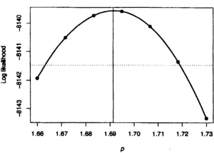
grid of values $bomp=1.66$ to$p=1.73$ in steps of0.01. A $sm\infty th$

cubic spline interpolationmaybefittedthrough$the\Re$computedpointsfor

amore

_accurate

estimate. Anominal coffidence interval for$p$ is found uslng that 2$\beta ogL[\hat{p})-\log L[Po)]$

$hu$, _{asymptotically,}

a

$\chi_{1}^{2}$ distribution, wheoe

$h$ is the true parmeter value. The profile

likehhood plot (Fig. 3) _indicates

_an

_{estimate of}$\hat{p}\approx 1.69$, with anomina195% conRdence

intervd $bom$ 1.663 _to 1.719 $appr\propto\dot{m}$ately. In practice, any value of$P$ in the (say) 95%

confldenoe intervd produce.$s$ very similar estimat$\infty$, models and residual plots. At this

empirical Bayesian estimate of$p$, compute $\hat{\beta}=0.0372,\hat{\tau}=0.376$and $\hat{\delta}=0.00173$

.

For each candidate vdue of $p$, numerical methods

are

used to $m\alpha i\dot{m}ze$ the

log-likelihood

over

the $(\beta,\delta)$ space, thenthe optimum vdue of$\tau$ fomd for each $(\beta,\delta)$

combi-nation. Theprocedure iteratu until convergence, and the entlre process repeated for the

next value of$p$ under consideration.

In particular, thevalue of$\beta$isof$inter\infty t$

.

The proffle$hkelih\infty d$plotfor$\beta$ (Fig. 4) shows

anomina195% confldenoe interW for $\beta$

,

computed sinilaely to that for

$p$, is&om 0.032

to 0.0427 apprnimately. This intervd certainly does not contain zero,

so

the $effe\alpha$ of

SOI is statistically $siffiiflcant,$ thoug the $Mue$ _{is small}

so

may _{not be of any} $pra\alpha ical$

signiflcance. In this cue, the $m\mathfrak{N}imumlikelih\infty d$ estimates

are

very $s$–lar to those

computed using the $emp\ddot{m}cal$ Bayesian approach (Tbble 2); this is $expe\alpha d$ since $\delta$ is

References

[1] CHEN,M.-H.

&IBRAHIM,

J. G. (2003). Conjugatepriors for generalized

_linear

models.

Statistica Sinica, 13, 461-476.

[2] DUNN, P. K. (2007). tweedie: Tweedie exponentialfamily models, $R$package.

Avail-able from http://cran._{r-proj ect.org/src/contrib/Descript$ions/tweedie$}

.

_ht

ml

[3] DUNN, P. K.

&SMYTH,

G. K. (2005).

Series

evaluation of

Tweedie

exponential

dis-persion models densities.

Statistics

and

Computing,

15,

267-280.

[4] DUNN, P. K.

&SMYTH,

G.

K. (2007). Evaluation of

Tweedie

exponent\’ial d\’ispers\’ion

model densities by Fourierinversion. Statistics and Computing, To appear.

[5] EFRON, B.

&MORRIS,

C. (1973). Stein’s estimation rule and its competitors–An

empirical Bayesapproach. Joumal

_of

the American Statistical Association, 68, 117-130.

[6] FERREIRA, P. E. (1982). Estimating equations in the presenoe of prior knowledge.

Biometnka, 69,

667-669.

[7] GAFFNEY, D. O. (1971). Seasonal rainfall Zones in Australia. Buitau

_of

Meteorology,

Working paper No 141.

[8] GELMAN, A., CARLIN, J. B., STERN, H. S.

&RUBIN,

D. B. (2003). Bayesian Data

Analysis, 2nd edn.

Boca Raton:

Chapman and Hall.

[9] GODAMBE, V. P.

&KALE,

B. K. (1991). Estimating

functions:

An overview. In

Estimatinghnctions, ed V. P. Godmbe, pp. $3rightarrow 20$

.

Oxford: Clarendon Press.

[10] IBRAHIM, J. G.

&CHEN,

$M.rightarrow H$

.

(2000). Powerpriordistributions for regression

mod-els. Statistical Science, 15, 46-60.

[11] JAMES, W.

&STEIN,

C. (1961). Estimation with quadratic loss. Proceedings

_of

the

Fourth Berkeley Symposium

on

Math. Statts$t$

.

and Probability, University ofCalifornia

Press, Berkeley, Vol. 1,

361-379.

[12] JRGENSEN, B. (1997) The Theory

_of

Dispersion Models. London: Chapman and

Hall.

[13]

K\"oPPEN,

W. (1931), Grundris$s$ der Klimakunde, 2nd edn. Berlin: De Gruyer.

[14] $McCuLLAGH$, P.

&NELDER,

J. A. (1989). Generalized linearmodels, 2nd edn.

Lon-don: Chapman and Hall.

[15] OHNISHI, T.

&TSUBAKI,

H. (2001). Minimization ofthe Fisher infomation matrix

under

a

given covarianoe matrix function. The Institute

_of

Stattstical Mathematics,

Research Memorandum No 819.

[16] OHNISHI, T.

&YANAGIMOTO,

T. (2007). Conjugate location-dispersion families.

Joumal

_of

the Japanese Stat\’istical Society, 37,

307-325.

[17] PIESSENS, R.

&DE

DONCKER-KAPENGA, E.,

\"UBERHUBER,

C. W. and KAHANER,

D. K. (1983). Quadpack: A Subroutine Package

_for

AutomaticIntqmtion,

Springer-Verlag: Berlin.

[18] R

DEVELOPMENT

CORE TEAM (2007). $R$: A language and environment for statistical

computing. R Foundation for StatisticalComputing, Vienna, Austria. ISBN

3-900051-07-0, URL http:$//www.R$_-project.org

[19] STONE, R. C.

&AULICIEMS,

A. (1992). SOI phase relationships with rainfall in

eastem Australia. Intemational Joumal

_of

Climatology, 12,

625-636.

[20] TROUP, A. J. (1965). The southern oscillation. The Quarterly Joumal

_of

the Royal

[21] TSUBAKI, H. (1988). A generalization of the quasi-likelihood and its application to

linear inferenoe (in Japanese). Doctorial dissertation, University

_of

Tokyo.

[22] TWEEDIE, M. C. K. (1984). An index which distinguishes between

some

important exponentialfmilies. Statistics: Applications and New Directions. Proceedings

_of

the

IndianStatistical Institute GoldenJubilee IntemationalConference, Indian

Statistical

Institute, Calcutta, pp. 579-604.

[23] YANAGIMOTO, T. &OHNISHI, T. (2005). Extensionsof

a

conjugate prior through the

Figure 1: The location of the

stations

in

the

study $-\overline{+}$ $\in\in^{-}$ $s$ $\overline{\overline{\hat{\frac{}{\urcorner 3}}\varpi\varpi\in}}-$ $\frac{\pi}{\succ 0}$ $\check{9}$ $s$論 tlon旧

1.66 167 168 169 170 171 172 173

$\rho$

Figure

3:

The profile

likelihood

plot

for

$p$

.

The

points represent the

actual

log-likelihoods

computed at the given values of $p$

.

The thick

solid

line

is

a

cubic

spline smooth through

the

computed points.

The dotted

horizontal line

represents

the

height of the nominal 95%

confidence

interval.

The

vertical line

is

the location

of the

empirical Bayesian

estimate

of

$p$

.

0.080 $0.\infty 5$ 0.040 0.045

$\beta$

Figure 4: The

profile

likelihood

plot for $\beta$

.

The thick solid line is the log-hkelihood. The

dotted

horizontal

line

represents

the

height

of the nominal 95% confidenoe interval. The

vertical line

is

the location of the

empirical

Bayesian

estimate of

$p$

.

Tbble

1:

Summaries

of the

total July

rainffil

(in millimetres) at

each station

5% 95%

Std

Percent

Station

${\rm Min}$ quantile

Median

Mean quantile _{${\rm Max}$} dev IQR

zeros

$\overline{400141.42.834.0l\delta 6.896.8}$

138.831.2

35.2

0.0

40024

$0$_の $0$ゆ

29.8

35.7

99.9

1596

350

398

80

40047

$0$_ユ 5_ユ 50_ユ

72.4

1786

5202

90.4

54.6

0.0

40075

00

1洛 30 瀞

37.7

1183

2266

₄₂₈

_23.9

_5.0

40079

$0$の $0$の

27.7

35.3

94.8

2580

45.7

25.3

8.0

40082

0.0

0.8

29.9

36.8

89.6

306.4

52.4

28.0

3.0

40083

$0$の $0$_の

28.2

35.3

99.4

224.2

419

297

30

40094

0.8

2 ユ 34ゐ

35.2

90.2

150.8

29.7

27.8

_0.0

40096

0.0

0.3

26.2

33.8

107.4

142.6

33.7

36.1

3.0

40104

0.0

0.0

34.8

35.5

107.9

137.7

33.5

32.4

8.0

40110

0.0

1.7

23.1

43.6

112.9

365.4

64.7

34.8

3.0

40117

1.0

4.0

65.4

84.9

228.4

879.9

145.5 42.7

0.0

40120

0.8

3.1

27.8

36.1

101.0

243.7

43.3

24.0

0.0

40124

0.0

$0$_の 24 あ

34.5

1142

2048

40.3

29.1

10.0

40167

0.0

1.1

53.4

90.9

245.2

885.4

142.6

54.8

5.0

40158

0.0

2.1

32.2

42.8

134.1

273.3

50.4

25.7

5.0

40160

12

55

50ゐ

66.8

178.5

367.3

67.8

61.8

0.0

40171

0.0

2.3

32.3

53.9

137.6

481.7

80.7

32.6

3.0

40184

0.8

1.4

29.0

37.9

104.8

228.1

42.0

38.5

0.0

40190

10

3 ゐ

58.8

72.7

_153.9

_406.2

_71.1

_62.0

_0.0

40196

0.7

3.8

64.2

71.8

178.3

363.4

71.2

69.0

0.0

40197

a.s

4.2

54.0

69.4

184.7

427.3

79.3

44.4

0.0

40224

0.1

2.6

32.4

51.9

149.2

404.0

72.0

27.8

0.0

40229

0.2

1.4

28.0

48.6

162.2

329.6

64.3

28.6

0.0

40231

0.0

3.5

36.1

54.9

153.5

435.6

77.0

44.0

3.0

40237

2 の 6の

300

54.1

1618

430.2

76.2

28.2

0.0

40242

04

34

31占

510

1429

4230

719

27.7

0.0

40244

0.2

4.9

31.2

52.5

159.4

378.8

68.8

27.3

0.0

40246

0.2

3.8

29.8

48.5

154.5

318.8

60.8

28.4

0.0

40257

12

5ゐ 58ゆ

887

2345

8671

1456

516

00

40382

0.0

1.8

40.2

41.2

109.0

212.1

41.1

34.2

3.0

41001

0.0

0.1

30.4

38.8

107.0

122.8

33.6

42.4

5.0

41011

0.0

0.4

30.8

31.9

75.7

128.5

28.3

30.4

3.0

41018

0.4

0.8

31.0

34.9

87.4

115.0

28.6

37.8

0.0

41022

2.3

4.3

45.2

49.3

141.3

158.3

40.2

48.6

0.0

41053

0.0

0.0

21

ユ 1

315

41056

1.6

2.6

316

392

41063

0.0

0.5

30.8

37.7

41072

0.0

0.0

25.0

33.3

41082

0.0

1.2

31.2

36.1

41083

0.0

0.6

31 の 0

401

41095

13

18

397452

41103

0.2

13

39.0

45.7

41116

2.0

3.1

34.4

45.0

41126

0.0

0.0

302332

833

1384

298

358

80

1043

1843

389

418

00

930

1314

316

399

30

761

1309

292

453

80

986

1374

326

362

50

1042

1249

336

476

50

1283

1438

364

39.7

00

1217

1587

393

532

00

1129

144.1

34.4

43.4

0.0

78.9

1222

287

371

100

Table

2:

Empirical

Bayesian

estimates and the maximum likelihood

estimates

for

fitting

the

model to July

rainfall

Empirical Bayesian Maximum likelihood

Parameter

estimate

estimate

$p$

169

$\beta$

0.0372

$\tau$ $0376$ $\delta$

0.00173

168

0.0371

0.369