Strained Vortex と 乱流の統計法則(計算流体力学に関わる数理的諸問題)

Strained

Vortex

と乱流の統計法則

“Strained

Vortex

and Statistical

Law

of

Turbulence”

神部勉、

畠山望

(

東大理

)

Tsutomu Kambe, Nozomu Hatakeyama

Department

of

Physics, University

of

Tokyo

August 30,

1996

Abstract

In recent computer simulations it is revealed that homogeneous

isotropic turbulence at high Reynolds number is regarded as the field

towhichtheintensevorticity structures, called ‘worms’,aredistributed

randomly [1, 2,3,4]. Itis also reported that ‘worm’ is approximated as

Burgers’ vortexunder external straining $[2, 4]$ and suchintense struc-ture causes intermittency [5]. So the statistical properties of a model

velocity field associated with an isolated Burgers’ vortex are studied.

It is found that, in suchamodel field, the 2nd-order structure function

shows the two-thirds law and the $3\mathrm{r}\mathrm{d}$-order structure function shows

the four-fifth law with a negative sign, which are consistent with the

Kolmogorov’s five-thirds law of theenergy spectrum and the negative skewnessof the velocity derivative respectively. Furthermore the

ex-ponentsofhigher-order structure functions arefound tobe consistent

1

Statistical

theory

of

homogeneous

isotropic

turbulence

1.1

Kolmogorov’s theory

(1941)

(1.5)

Let the velocity components $v_{i}(x)$ at each location $x$ be center-valued

ran-dom variables, while the brackets $\langle(\cdot)\rangle$ denote the ensembleaverage. We

con-sider the instantaneous statistics of the velocity fluctuations at a fixed time.

The center valued property $\langle v_{i}\rangle=0$ can be satisfied by means of Galilean

transformations which are symmetries of the Navier-Stokes equation,

$\frac{\partial v}{\partial t}+v\cdot\nabla v=-\frac{1}{\rho}\nabla p+\nu\triangle v$, (1.1)

$\nabla\cdot v=0$, (1.2)

where $\rho$ is the mass density, $p$ the pressure and $\nu$ the kinematic viscosity.

We consider now turbulence of homogeneous and isotropic velocity field.

The longitudinal velocity increment for the separation $l$ and the pth-order

$l_{on}gitudoeinal$ structure

function

are respectively defined as

$\delta v\ell(X,l)\equiv\delta v(X,l)\cdot\frac{l}{l}$, (1.3) $s_{p}(l)\equiv\langle(\delta vt(_{X,l}))^{p}\rangle$ , (1.4)

where $l\equiv|l|$. The dependence of $S_{p}$ on _$x$ and $l/\ell$ is dropped because of

homogeneity and isotropy. One reason why we consider the longitudinal

component is that, in the 2nd- and $3\mathrm{r}\mathrm{d}$-order case, the structure functions made of other components are determined by the longitudinal one.

We introduce the mean energy dissipation rate $\epsilon$ defined as, in Cartesian coordinate system,

$\epsilon\equiv\langle\frac{1}{2}\nu\sum_{ij}(\frac{\partial v_{i}}{\partial x_{j}}+\frac{\partial v_{j}}{\partial x_{i}}\mathrm{I}^{2}\rangle$,

and the $I\mathrm{e}’olmogorov$ dissipation scale $\eta$ as, using $\nu$ and $\epsilon$,

$\eta\equiv(\nu^{3}/\epsilon)^{1/4}$ (1.6)

Kolmogorov(1941) made thenext two hypotheses in the case of homogeneous

Kolmogorov’s hypothesis ofsimilarity I In the range

_of

scales $l\ll\eta$

which is called the dissipationrange, all the statisticalproperties are uniquely

determinedby the scale$\ell$, the viscosity$\nu$ andthe mean energydissipationrate $\epsilon$.

Kolmogorov’s hypothesis of similarity II In the range

_of

scales $\ell\gg\eta$

which is called the inertial range, all the statistical properties are uniquely

determined by $\ell$ and $\epsilon$ only.

The $2\mathrm{n}\mathrm{d}$-order longitudinal structure function is obtained from the above

hypotheses as

$S_{2}( \ell)=\frac{\epsilon}{15\nu}\ell 2$ $(\ell\ll\eta)$ (1.7)

$=C\epsilon^{2}l^{2}/3/3$ _$(l\gg\eta)$, _(1.8)

where$C$ is auniversal dimensionless constant. Thebehaviorofthe $2\mathrm{n}\mathrm{d}$-order

structure function as the two-thirds power of the distance in the inertial

range is called the two-thirds law, which holds experimentally for almost any

turbulence [7]. This law corresponds to the

_five-thirds

law of the energy

spectrum.

The $3\mathrm{r}\mathrm{d}$-order longitudinal structure function becomes

$S_{3}( \ell)=-\frac{4}{5}\epsilon\ell+6\nu\frac{dS_{2}(l)}{d\ell}$, (1.9)

which is derived from the incompressible Navier-Stokes equation (1.1) and

(1.2) [8]. In the inertial range $\ell\gg\eta$, the second term of (1.9) is dropped

on account of Kolmogorov’s second hypothesis, and so-called

_four-fiflh

law is

obtained as

$S_{3}( \ell)=-\frac{4}{5}\epsilon\ell$ _{$(\ell\gg\eta)$}. (1.10)

For the higher-order structure functions, the following is said from the

Kolmogorov’s second hypothesis. Let $S_{p}(\ell)$ be the $p\mathrm{t}\mathrm{h}$-order longitudinal

structure function,

$S_{p}(l)=C\epsilon^{p/}\ell p3p/3$ $(\ell\gg\eta)$, (1.11)

where $C_{p}$ is the universal dimensionless constant. In general $S_{p}(\ell)$ is

repre-sented in the form of scaling law with the scaling exponent $\zeta_{p}$ as

Thus the exponent $\zeta_{p}$ of the Kolmogorov’s theory (K41) is, from (1.11),

$\zeta_{p}=\frac{p}{3}$. (1.13)

Experimentally and in the DNS, it is found that $\zeta_{p}$ increase less rapidly

with $p$ than the K41 value of (1.13). This fact is called anomalous

scal-ing in the inertial range, which means the stronger fluctuations to exist in

the smaller scales. Thus the various intermittency models subject to some

statistics of the velocity increment or the local dissipation have been

sug-gested after K41, which are summarized in Frisch [7].

1.2

Multifractal model

Parisi and Frisch (1985) presented the

_multifractal

model in the following

way [9]. Assuming that, in the limit of infinite Reynolds number, there is a

set $S_{h}\subset R^{3}$ of the

fractal

dimension $D(h)$ for each velocity scaling exponent $h$ as $\ellarrow 0$, that is,

$\delta v_{\mathit{1}}(X)\propto\ell^{h}$, _{$x\in S_{h}$}. (1.14)

From this

_multifractal

assumption, the $p\mathrm{t}\mathrm{h}$-order structure function is ex-pressed as

$S_{\mathrm{p}}(\ell)$ oc $\int d\mu(h)^{\ell^{p+\langle h)}}h3-D$, (1.15)

where $d\mu(h)$ isthe measurewhichgivestheweight ofthedifferent exponents.

In the limit $larrow \mathrm{O}$ the power-law with the smallest exponent dominates, thus

$\zeta_{p}=\min_{h}(ph+3-D(h))$

.

(1.16)

1.3

${\rm Log}$

-Poisson

model

The $log$-Poisson model with no adjustable parameters was proposed recently

by She et al.(1994) first based on a phenomenology involving a hierarchy

offluctuation structures associated with vortexfilaments, and later the

log-Poisson property was noted by Dubrulle (1994) and She et al. (1995)

inde-pendently [10]. The resulting exponent

$\zeta_{p}=\frac{p}{9}+2-2(\frac{2}{3})^{p/3}$ (1.17)

is ingood agreementwiththeresult of the experiment by Anselmet et al. [11],

2

A

model-vortex field

2.1

Burgers’ vortex

We consider a model-field of isolated Burgers’ vortex whose circulation and

axial stretching rate are the typical values in homogeneous isotropic

turbu-lence, and investigate the structurefunctions of this field.

In the cylindrical coordinate system $(r, \theta, z)$, let the axisymmetric

vortic-ity along $z$ axis$\omega$and the velocity associated with vorticity$v_{\mathrm{t}p}$ berespectively

$\omega=(0,0,\omega(r))$, (2.1)

$v_{\omega}=(\mathrm{O}, v_{\theta}(r),$ $\mathrm{o})$, (2.2) where $\omega=dv_{\theta}/dr+v_{\theta}/r$

.

Imposing the straining of the irrotational and

solenoidal velocity field

$v_{\mathrm{e}}=(- \frac{\sigma}{2}r,0, \sigma z)$, (2.3)

the total velocity $v=v_{\omega}+v_{e}$ is given as

$v=(- \frac{\sigma}{2}r,v_{\theta}(r),\sigma \mathcal{Z})$, (2.4)

where $\sigma$ is a positive constant. The vorticity equation reduced from the

incompressible Navier-Stokes equation (1.1) and (1.2),

$\frac{\partial\omega}{\partial t}+v\cdot\nabla\omega=\omega\cdot\nabla v+\nu\triangle\omega$, (2.5)

has the exact steady solution in the form

$\omega(r)$ $= \omega_{0}\exp(-\frac{\sigma r^{2}}{4\nu})$ $= \frac{\Gamma}{\pi r_{\mathrm{B}}^{2}}\exp(-\frac{r^{2}}{r_{\mathrm{B}}^{2}})$ , (2.6)

$v_{\theta}(r)$ $= \frac{2\nu\omega_{0}}{\sigma r}\{1-\exp(-\frac{\sigma r^{2}}{4\nu})\}=\frac{\Gamma}{2\pi r}\{$$1- \exp(-\frac{r^{2}}{r_{\mathrm{B}}^{2}})\},$ $(2.7)$

where the Burgers’ radius$r_{\mathrm{B}}$ defined as $1/e$ radius of$\omega(r)$ is

and the circulation $\Gamma$ is

$\Gamma\equiv\int_{0}^{\infty}\omega(r)2\pi rdr=\pi r_{\mathrm{B}}^{2}\omega_{0}$. (2.9)

This is called the Burgers’ vortex [12]. TheBurgers’ vortex is also the

asymp-totic solution for the arbitrary initial axisymmetric vorticity distribution in the case of uniform strain as is $\mathrm{a}\mathrm{b}\mathrm{o}\mathrm{v}\mathrm{e}[13]$.

The rate

_of

strain tensors defined as, in theCartesian coordinate system,

$e_{ij}(x) \equiv\frac{1}{2}(\frac{\partial v_{i}}{\partial x_{j}}(x)+\frac{\partial v_{j}}{\partial x_{i}}(x))$ , (2.10)

is calculated as $e=($$\frac{1}{2}(_{d^{-}r}^{\underline{d}_{\Delta}v}vr_{0}\frac{\sigma}{2}-^{\Delta})$ $\frac{1}{2}(\frac{dv}{d}r^{\mathrm{A}}-\frac{\sigma}{2}r0-^{\Delta}v)$ $\sigma 0$

)

$0$

.

(2.11)

The axial stretching rate of vorticity has a positive constant value as

$\frac{\Sigma_{ij}\omega_{i}(r)e_{i}j(r)\omega j(r)}{\Sigma_{k}\omega_{k}^{2}(r)}=\sigma$ . (2.12)

The squared strength of $e$ is evaluated as a function of $r$,

$e^{2}(r) \equiv\sum ije^{2}ij(\Gamma)=\frac{3}{2}\sigma^{2}+\frac{1}{2}(\frac{dv_{\theta}}{dr}(r)-\frac{v_{\theta}(r)}{r}\mathrm{I}^{2}$ , (2.13)

thus the local energy dissipation rate is given as

$\mathcal{E}_{1\mathrm{o}\mathrm{c}}(r)\equiv 2\nu e(2)r=\nu\{3\sigma^{2}+(\frac{dv_{\theta}}{dr}(r)-\frac{v_{\theta}(r)}{r}\mathrm{I}^{2}\}\cdot$ (2.14)

Because the azimuzal velocity profile is obtained by (2.7),

$\frac{dv_{\theta}}{dr}(r)-\frac{v_{\theta}(r)}{r}=\frac{\Gamma}{\pi r_{\mathrm{B}}^{2}}\{\exp(-r^{2}/r_{\mathrm{B}}^{2})-\frac{1-\exp(-r2/r_{\mathrm{B}}^{2})}{r^{2}/r_{\mathrm{B}}^{2}}\}$

.

(2.15)

If $\Gamma$ is large enough

in comparison with $\sigma$, theenergy ofthe Burgers’ vortex

is strongly dissipated around the Burgers’ radius while at the center of vortex

$\mathrm{r}/\mathrm{r}_{\mathrm{B}}$

Figure 1: Dashed line, theaxial vorticity$\omega$; dotted line, theazimuthal

veloc-ity $v_{\theta}$; solidline, the localenergy dissipation rate $\epsilon_{1\mathrm{o}\mathrm{c}}$ of the Burgers’ vortex. $r_{B}=1,$ $\nu=0.1$ and $R_{\Gamma}\equiv\Gamma/\nu=1257$.

2.2

Calculation

Calculationofaverageof the velocity increment between two separated points

is as follows, suggested first by Kambe et al. [14]. First choose a reference

point $x=(x,0, z)$ in the Cartesian coordinate system, where the dependence

on the $y$ component can be dropped from the axisymmetry of the velocity

field, and choose a running point $x+l$ at a distance $l$ from _$x$

.

Next the

velocity increment between the two points is calculated. Last, the average

of the $p\mathrm{t}\mathrm{h}$-order longitudinal velocity increment over the sphere of radius $\ell$

centered at $x$ is taken, and then volume averaging is carried out by shifting

the reference point.

Let the location on the spherical surface centered at the reference point

$x$ be$l=(\ell, \theta, \phi)$ in the spherical coordinate system as shown in figure 2 (a).

The components of $l$ in the Cartesian coordinate system are written as

Figure2: (a) The coordinate system at spherical

average

with respect to the

running point $x+l$ where the reference point $x$ and the separation length$\ell$

are fixed. (b) The integral space with respect to $\mathrm{t}1_{1}\mathrm{e}$ reference point

$x$

.

The longitudinal velocity increment $\delta v\ell(x,l)$ is calculated from the equations

(1.3) and (2.7) as

$\delta v_{\ell}(x,\ell,\theta, \phi)=\sigma\ell\frac{3\cos^{2}\theta-1}{2}+(\frac{v_{\theta}(r)}{r}-\frac{v_{\theta}(x)}{x}\mathrm{I}x\sin\theta\sin\phi$

$= \frac{\nu}{r_{\mathrm{B}}}[\frac{4\ell}{r_{\mathrm{B}}}P_{2}(\cos\theta)+\frac{R_{\Gamma}}{2\pi}\{\frac{1-\exp(-r^{2}/r_{B}^{2})}{r^{2}/r_{B}^{2}}$

$- \frac{1-\exp(-X/2)r_{B}^{2}}{\mathrm{t}^{2}/\Gamma_{B}^{2}}.\}\frac{x}{r_{\mathrm{B}}}\sin\theta\sin\phi]$

,

(2.17)

$r^{2}=(x+\ell\sin\theta\cos\phi)2+(\ell\sin\theta\sin\phi)2$, (2.18)

where $P_{2}$ is the second-order Legendre function and $R_{\Gamma}=\Gamma/\nu$ is the Vortex

Reynolds number based on its total circulation. Note that a dependence on

$z$ is dropped in the expression at this moment. The spherical

averag.e

is thus

calculated as

Choosing some region of space as a sample space, we take an average $\langle(\cdot)\rangle$

over the space. One sample is the cylindrical space of radius $r_{\mathrm{c}}$ centered at

the vortex axis shown in figure 2 (b). In the cylindrical coordinate system

$(r,\theta, z)$, the average is

$\langle$$( \cdot))\equiv\lim_{z_{\mathrm{c}^{arrow}}\infty}\frac{1}{2\pi r_{c}^{2_{Z_{\mathrm{C}}}}}\int_{-z_{\mathrm{C}}}^{z_{\mathrm{C}}}\int_{-\pi}^{\pi}\int_{0}^{r_{\mathrm{C}}}(\cdot)rdrd\theta dz$. (2.20)

The $p\mathrm{t}\mathrm{h}$-order longitudinal structure function is given as follows,

$S_{p}(l, r_{\mathrm{C}}) \equiv\frac{2}{r_{\mathrm{c}}^{2}}\int_{0}^{r_{\mathrm{C}}}((\delta v_{l})p\rangle_{\mathrm{s}\mathrm{p}}XdX$

.

(2.21)

$10^{6}$ $10^{4}$ $-\mathrm{S}_{3}10^{8}$ $10^{0}$ $10^{-2}$ $1/\mathrm{r}_{\mathrm{B}}$

Figure 3: The $3\mathrm{r}\mathrm{d}$-order structure function times-l. $\mathrm{O},$ $R_{\Gamma}=628;\square ,$ $R_{\Gamma}=$

1257; and $,$ $R_{\Gamma}=12566$

.

The structure functions are calculated at $R_{\Gamma}=628,1257$ and 12566.

are shown. The inertial range begin around $\ell\sim r_{B}$ and is wider as $R_{\Gamma}$ is

larger. It is found that the $3\mathrm{r}\mathrm{d}$-order exponent

$\zeta_{3}$ is about unity

indepen-dent of $R_{\Gamma}$. This scaling is consistent with Kolmogorov’s four-fifth law. In

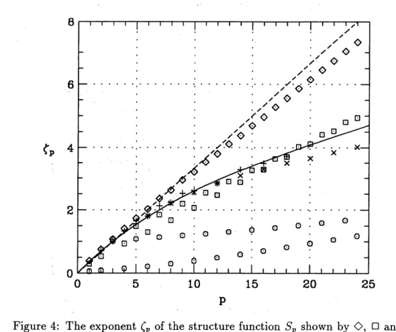
the figure 4 other exponents $(_{p}$ up to $p=25$ are shown in comparison with

K41, $\log$-Poisson model, DNS and experiment. The lager $R_{\Gamma}$ is, the more $\zeta_{p}$

deviates from K41. The tendency of the even exponents to extend the odd

ones in this model is the same in the experiment by Anselmet et al..

$\zeta_{\mathrm{p}}$

$\mathrm{p}$

Figure 4: The exponent $\zeta_{p}$ of the structure function $S_{p}$ shown by $\mathrm{O},$ $\square$ and

${ }$ which are as in figure 3. dashed line, K41 (1.13); solid line, log-Poisson

model (1.17); $\cross$, DNS at $R_{\lambda}=150$, Vincent&Meneguzzi (1991) [1]; _$+$, jet

at $R_{\lambda}=852$, Anselmet et al.(1984) [11].

If the vortex is absent, therefore $v_{\theta}=0$, we have $S_{p}(\ell)=C_{p}\sigma^{p}\ell^{p}\propto\ell^{p}$

if the external strain is absent so that $\sigma=0$, we find that the structure

functions of odd order are identically zero by use of(2.7), (2.18) and (2.19).

Hence the scaling consistent with the homogeneous isotropic turbulence as

obtained above is considered to result from the combined field of the vortex

under external straining.

The probability distribution functions of the vortex Reynolds number$R_{\Gamma}$ and the Burgers’ radius $r_{B}$ of worms are obtained by Jimen\’ez et al. [2] in

DNS and by Belin et al. [5] experimentally. Especially $R_{\Gamma}/R_{\lambda^{/2}}^{1}$ distributes

independent of$R_{\lambda}$. Taking that $\mathrm{p}.\mathrm{d}$.f.s into account we expect to obtain the scaling nearer that of experiments which is K41 like scaling of low-order at any $R_{\lambda}$ and the higher-order scaling with the larger deviation from K41.

3

Summary

The conclusions of this study are $\mathrm{S}\mathrm{U}\mathrm{n}\mathrm{m}\mathrm{l}\mathrm{a}\mathrm{r}\mathrm{i}_{\mathrm{Z}\mathrm{e}\mathrm{d}}$as follows.

1. This model field of the isolated Burgers’ vortex withmoderate circula-tion shows that the $2\mathrm{n}\mathrm{d}$-order structure function has about two-thirds

scaling exponent.

2. The $3\mathrm{r}\mathrm{d}$-order structure function of this model have anegativesign and unity exponent independent of the vortex Reynolds number $R_{\Gamma}$

.

3. The scaling exponents of the high-order structure function obtained

from the model-strained vortex field deviates increasingly from K41 as

$R_{\Gamma}$ is larger, i.e. a Burgers’ vortex causes moreand more intermittency of turbulence as it’s circulation is larger.

References

[1] A. Vincent and M. Meneguzzi, J. Fluid Mech. 225, 1-20 (1991).

[2] J. Jimen\’ez, A. A. Wray, P. G. Saffman and R. S. Rogallo, J. Fluid Mech.

255, 65-90 (1993); J. Jimen\’ez and A. A. Wray, CTR Annual Res. Briefs,

287-312

(1994).

[3] 山口博、 生出伸$-\text{、}$ 山本稀物、細川巌、第

9

[] 数値流体力学シンポ

[4] 店橋護、宮内敏雄、吉田毅、第9o 数値流体力学シンポジウム講演論

文集、pp. 171-172 (1995).

[5] F. Belin, J. Maurer, P. Tabeling, H. Willaime, J. Phys. II France 6,

573-583 (1996).

[6] A. N. Kolmogorov, C. R. Acad. Sci. USSR30,

301-305

(1941); ibid. 32,

16-18 (1941).

[7] U. Frisch, Turbulence (Cambridge U.P., Cambridge, 1995).

[8] L. D. Landau and E. M. Lifshits, Fluid8 Mechanics, 2nd edition

(Perg-amon Press, Oxford, 1987),

_{\S 34.}

[9] G. Parisi and U. Frisch, in Turbulence and Predictability in Geopysical Fluid Dynamics, edited by M. Ghil, R. Benzi and G. Parisi (Amsterdam,

North-Holland, 1985), pp.

84-87.

[10] Z. -S. She and E. Leveque, Phys. Rev. Lett. 72, 336-339 (1994); B.

Dubrulle, ibid. 73,

959-962

(1994); Z. -S. She and E. C. Waymire, ibid.

74, 262-265 (1995).

[11] F. Anselmet, Y. Gagne, E. J. Hopfinger and R. A. Antonia, J. Fluid

Mech. 140, 63-89 (1984).

[12] J. M. Burgers, Adv. in Appl. Mech. 1, 171-199 (1948).

[13] T. Kambe, J. Phys. Soc. Jpn. 53, 13-15 (1984).

[14] T. Kambe and I. Hosokawa, in Small-Scale Structures in

Three-Dimensional Hydrodynamic and Magnetohidrodynamic Turbulence,

edited by M. Meneguzzi, A. Pouquet and P. L. Sulem (Springer-Verlag,