経済構造分析におけるグラフ最適化とネットワーク指標に関する研究

(1)

Kyushu University Institutional Repository

経済構造分析におけるグラフ最適化とネットワーク指標に関する研究

土中, 哲秀

https://doi.org/10.15017/1931691

出版情報：Kyushu University, 2017, 博士（経済学）, 課程博士バージョン：

権利関係：

(2)

Studies on

Graph Optimization and Network Indicators in Economic Structure Analysis

Thesis by

Tesshu Hanaka

In Partial Fulfillment of the Requirements for the Degree of

Doctor of Philosophy

Kyushu University

Graduate School of Economics, Hakozaki, Fukuoka, Japan February, 2018

(3)

Preface

In the field of economic structure analysis, a nature of economy as a network has been focused on. A network is a discrete structure that consists of (weighted) vertices and (weighted) edges that connect vertices. In the context of economic analysis, vertices represent industries, sectors, companies or individuals, and edges represent transactions between them. In weighted cases, the weight of a vertex or an edge represents its magnitude. For example, if a vertex corresponds to an industry, its production volume is represented as the vertex weight, and if an edge corresponds to a transaction between two industries, the amount of money or materials transferred between them is represented as the edge weight.

In general, a graphical/network representation gives an intuitive observation about the lo- cal/global structure of connections. Thus a typical usage of economic network model is to identify a group of industries/transactions that play a key role in economy. This type of analyses are also useful to capture flow of certain things on a network. In fact, in the field of environmental economics, economic network analysis is used to discover industries and transactions with high environmental burden of pollutants caused by economic activities.

The network analysis methods are roughly categorized into two approaches. One is graph optimization approach, and the other is network indicator approach. The graph optimization approach works as follows: We first model the task of analysis as a graph optimization problem. We then apply an algorithm to solve the problem, and obtain a solution. The solution implies analytical results about the network to be considered.

The network indicators reflect the characteristics of the network. Typically, these indicators are defined for vertices and/or edges, which represent their importance. The network indicator approach quantitatively argues the features of the network via the indicators.

These approaches have been applied to economic network analysis and they are promising in the

(4)

field of economic structure analysis. In this thesis, we reorganize and develop the graph optimization approach and the network indicator approach from the viewpoint of economic structure analysis.

February, 2018 Tesshu HANAKA

(5)

Acknowledgments

First of all, I would like to express my sincere appreciation to my supervisor, Professor Hirotaka Ono of Nagoya University for his unconditional support from the beginning to the end. He kindly gave me his deep knowledge, insightful suggestions, and generous encouragement. He also taught me that research is very exciting and pleasant. I am deeply grateful to him for his polite and persistent guidance. A lot of valuable experience he granted to me will become an irreplaceable treasure in my life. Without his dedicated help, I would never complete this dissertation.

I wish to express my deepest appreciation to Professor Shigemi Kagawa of Kyushu University for being a great adviser to me. He gave me his deep insight and extensive knowledge. I am indebted to him for his constructive advice and warm encouragement.

I would also like to express my deep gratitude to my committee members, Professor Tetsuya Furukawa and Professor Toshio Ohnishi of Kyushu University for their generous support and helpful comments.

My heartfelt gratitude goes to Professor Hans L. Bodlaender of Utrecht University, Professor Naomi Nishimura of University of Waterloo, Professor Keiichiro Kanemoto of Shinshu University, and Mr. Tom van der Zanden of Utrecht University for their kind cooperation as coauthors. I have greatly benefited from their scientific expertise, and their generous help and advice advanced my research.

I would like to thank Professor Eiji Miyano of Kyushu Institute of Technology, Professor Ya- sushi Kondo of Waseda University, Professor Yota Otachi of Kumamoto University, Professor Toshiki Saitoh of Kyushu Institute of Technology, Professor Yen Kaow Ng of Universiti Tunku Abdul Rahman, Professor Michael Lampis of Université Paris-Dauphine, Professor Jesper Nederlof of Eindhoven University of Technology, Professor Johan M. M. van Rooij of Utrecht University, Professor Hiroshi Eto of Kyushu University, Mr. Ioannis Katsikarelis of Université Paris-Dauphine,

(6)

and Mr. Krishna Vaidyanathan of University of Waterloo for many enlightening discussions.

It is impossible to conclude my acknowledgment without all the members of Ono laboratory.

Since I started my research life, Dr. Omar Rifki and Mr. Petar Tzenov have supported me as my colleagues and my friends. The remaining members of Ono laboratory have also given me fulfilling days.

I would also like to thank Professor Yasunori Hanamatsu, Mr. Shota Tokunaga, and the remaining members of Decision Science for a Sustainable Society of Kyushu University for their constructive help.

Finally, but not least, I would like to thank my family, my mother, my father and my siblings.

Without their care, support and encouragement, this dissertation would not have been possible.

(7)

List of Figures

2.1 An undirected graph . . . 11

2.2 A directed graph . . . 11

2.3 A graph (left) and its tree decomposition of width two (right) . . . 16

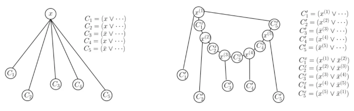
3.1 Original clauses wherex’s appear . . . 23

3.2 Replaced clauses . . . 23

3.3 Constructed graph of the reduction from 3SAT to(0,1)-EDS . . . 25

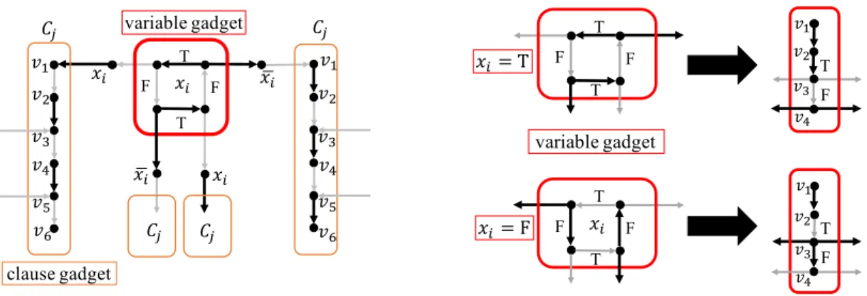
3.4 Replacing a cycle by a directed path for a variable’s gadget . . . 25

3.5 Vertex gadgets forvwithdⁱⁿ(v) = 2in the reduction to(1,1)-EDS . . . 27

3.6 Vertex gadgets forvwithd^out(v) = 2in the reduction to(1,1)-EDS . . . 27

3.7 Replacing an edge and attaching path gadgets for the reduction to(p, q)-EDS . . . 29

3.8 Replacinge= (u, v)by a gadget forr-VC . . . 30

3.9 Replacinge= (u, v)by a gadget for(0, q)-EDS . . . 30

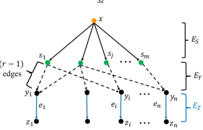
3.10 Constructed graph of the reduction from SET COVERto DIRECTEDr-OUT VER- TEXCOVER . . . 32

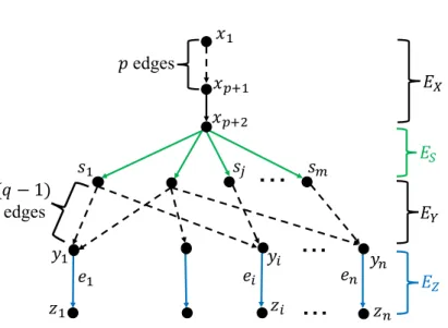
3.11 Constructed graph of the reduction from SET COVER to DIRECTED (p, q)-EDGE DOMINATINGSET . . . 34

4.1 Connection between vertex sets . . . 68

5.1 An example of the vertex betweenness centrality for sectorv . . . 86

5.2 An example of the edge betweenness centrality for transaction(u, v) . . . 89

5.3 Consumption-based CO2emissions of each country . . . 94

5.4 CO₂emission transfer of each country . . . 95

(11)

5.5 Rank correlation of vertex betweenness centrality indices between CO₂ emissions and energy consumptions associated with the final demand in each demand country 96 5.6 High-priority supply-chain network with higher edge betweenness centrality for

CO2emissions associated with the final demand in the U.S.A. (circle size indicates amount of vertex betweenness centrality and edge width indicates amount of edge betweenness centrality) . . . 104 5.7 High-priority supply-chain network with higher edge betweenness centrality for

CO2 emissions associated with the final demand in Germany (circle size indicates amount of vertex betweenness centrality and edge width indicates amount of edge betweenness centrality) . . . 105

(12)

List of Tables

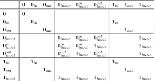
3.1 Our results for graph classes. NP-c andW[2]-h stand for NP-complete andW[2]- hard, respectively. Note thatγ = max{p, q}and∆ = maxv∈V(dⁱⁿ(v) +d^out(v)). 19 3.2 Entries indicate case numbers that apply for the possible states ofu andv for the

introduce node for the edge(u, v). The labels for the rows correspond toc(u)and the labels for the columns correspond toc(v). . . 49 3.3 Entries indicatec_i(v)for possible combinations ofc_j₁(v)andc_j₂(v)forvin a join

nodeiwhich has two children nodej1andj2. . . 53 3.4 Entries indicate case numbers that apply for possible states ofuandvfor the intro-

duce node for the edge(u, v). The labels for the rows correspond toc(u) and the labels for the columns correspond toc(v). . . 54 4.1 This table represents combinations of states of two child nodes j1, j2 for each

vertex in X_i = X_j₁ = X_j₂. The rows and columns correspond to states of j₁, j₂ respectively and inner elements correspond to states of x. For example, if ci(v) = sA, there are three combinations such that (cj1(v), cj2(v)) = (sA, s∅), (c_j₁(v), c_j₂(v)) = (s_∅, s_A)and(c_j₁(v), c_j₂(v)) = (s_A, s_A). . . 73 4.2 Combinations of the original coloring in join node . . . 82 4.3 Combinations of the new coloring in join node . . . 82 5.1 Top 30 sectors for vertex betweenness centrality (VB) for CO2 emissions in the

global supply-chain networks associated with the final demand in each demand country . . . 98 5.2 Top 30 sectors of vertex betweenness centrality (VB) for CO₂ emissions in the

global supply-chain network associated with the global final demand . . . 99

(13)

5.3 Top 30 transactions for edge betweenness centrality (EB) for CO₂ emissions in the global supply-chain networks associated with the final demand in each demand country . . . 100 5.4 Top 30 transactions of edge betweenness centrality (EB) for CO2emissions in the

global supply-chain network associated with the global final demand . . . 101 A.1 Industry classification of the World Input-Output Table (WIOT) . . . 111 A.2 Country classification of the World Input-Output Table (WIOT) . . . 112 B.1 Top 30 sectors of vertex betweenness centrality (VB) for energy consumptions in

the global supply-chain network associated with the global final demand . . . 114 B.2 Top 30 sectors of vertex betweenness centrality (VB) for energy consumptions in

the global supply-chain networks associated with the final demand in each demand country . . . 115 B.3 Top 30 transactions of edge betweenness centrality (EB) for energy consumptions

in the global supply-chain network associated with the global final demand . . . . 116 B.4 Top 30 transactions of edge betweenness centrality (EB) for energy consumptions in

the global supply-chain networks associated with the final demand in each demand country . . . 117 B.5 The comparison of Top 30 sectors of vertex betweenness centrality between CO2

emissions and energy consumptions in the global supply-chain network associated with the global final demand . . . 118 B.6 The comparison of Top 30 sectors of vertex betweenness centrality between CO2

emissions and energy consumptions in the global supply-chain network associated with the final demand in each demand country . . . 119 B.7 The comparison of Top 50 transactions of edge betweenness centrality between CO₂

emissions and energy consumptions in the global supply-chain network associated with the global final demand . . . 120 B.8 The comparison of Top 30 transactions of edge betweenness centrality between CO2

emissions and energy consumptions in the global supply-chain network associated with the final demand in each demand country . . . 121

(14)

Chapter 1

Introduction

1.1 Background

A network is a pattern of interconnections among a set of things [21]. It consists of some objects, calledvertices ornodes, and some pairs of the objects, called edges orlinks. Networks can express any “relationships” or “connections”. Typical examples are computer networks, which represent the connection between computers, the World Wide Web, which represent the connections between web pages, traffic networks, in which vertices represent intersections or stations and edges represent roads or rails, friendship networks, which consist of vertices of persons and edges between them, and trade networks in which vertices represent industries or companies and edges represent direct transactions [21,86,87]. Also bioinformatics uses protein-protein interaction networks, which represent the physical contacts between proteins in the cell [47, 99].

By expressing a set of relations as a network, we can intuitively understand structures of relations. For example, by using social networks, we can observe how complicated human relations are, who is a key person in the group, which relationship between persons is strong, and so on. We can also find which route is the shortest in a map by using transportation networks, and analyze transaction structures among industries by using trade networks. As above, observing networks gives us a lot of insight and /or deep understanding.

On the other hand, the amount of information in the world rapidly increases nowadays, and many networks become large and complicated. Consequently, it gets harder and harder to observe the structure and the property of a network. To solve this situation, it is required to observe the

(15)

network by extracting the key structure, or developing indicators that reflect the structures without seeing the whole network.

For this, network analysis is studied in many research fields for a long time. Network analysis is a research method that analyzes the structures and properties of a network by using mathematical tools such as graph theory, linear algebra, and so on. Among them, thegraph optimization approach is a typical approach of network analysis. This approach uses graph optimization problems and algorithms for solving them. Another well-known approach isnetwork indicator approach, which uses indicators that represent the characteristics of a network.

In this thesis, we develop analytical methods for economic networks based on the graph optimization approach and the network indicator approach. An economic network consists of vertices corresponding to industries, sectors or companies and edges corresponding to transactions. That is, an economic network represents the economic structure and analyzing the economic network leads to the grasp of economic structure. Consequently, economic network analysis is useful to carry out appropriate economic policies and managements.

1.1.1 Graph optimization approach

In mathematical literature, a network is often called agraph. The graph optimization approach is a typical network analysis approach based on graph optimization problems and algorithms. In the graph optimization approach, we first model the task to discover a critical structure as a graph optimization problem. We then solve the problem by using the algorithm and obtain the desired structure.

For example, given a map, a person would like to go to the destination as fast as possible, he or she needs to take the “best” route on the map. How can he/she find such a route? This can be done by using the graph optimization approach: First, we describe the map as a graph. Next, we model the task to find an optimal route in the map as a graph optimization problem. In an edge- weighted graph, ashortest pathfromstotis defined as a path fromstotwith minimum weight.

The weight of an edge represents the distance between two points. The task to find an optimal route can be modeled as the graph optimization problem to find a shortest path. This problem is called the SHORTEST PATHproblem [25]. Finally, by solving the SHORTEST PATH problem, we can obtain an optimal route in the map.

(16)

A shortest path is one of the important graph structures, and there are other structures in the graph as well. In a graph, aseparatoris a subset of vertices that divides the graph into two parts.

Similarly, acutis a subset of edges that divides the graph into two parts. The problems to find a minimum separator and a minimum cut are well-studied as MINIMUMSEPARATORand MINIMUM

CUT, respectively. Finding a minimum separator and a minimum cut correspond to finding a bottle- neck in the network. Also, when a cut is small, the two divided sets are less related in the sense. By dividing a network with minimum cuts iteratively, we can detect the dense structures that implies strong relations between vertices, so-called communities in the network. Splitting a large network into subnetworks also makes it easier to observe the network structure. The division of the network is used in various aspects such as community analysis, image segmentation, and so on [36,101,102].

The generic name of that method isgraph clustering. The task is grouping the vertices of the graph into subsets of them, called clusters, such that there exist few edges between clusters [101]. A lot of clustering methods have been proposed since the criteria of goodness of division depends on the type of networks. Some of them are based on the graph optimization approach, such as finding minimum cuts iteratively [17, 26, 46, 50, 73, 102, 104, 115].

In the graph optimization approach, we need to design the algorithm to solve the corresponding graph optimization problem if any good algorithm is not known. From the aspect of algorithm design, the running time is a critical factor to obtain a solution at high speed. If a problem has a polynomial-time algorithm, it can be solved in realistic time as one theoretical criteria. In fact, polynomial-time algorithms are useful in practice. For example, SHORTESTPATH, MINIMUMSEP-

ARATOR, and MINIMUMCUThave polynomial-time algorithms [25, 35].

On the other hand, if there is no polynomial-time algorithm for a problem, it may not be solved in realistic time when the size of input is large. Actually, there exist a lot of problems that are anticipated to have no polynomial-time algorithm, which are known as NP-hard (or NP-complete) problems. For example, FEEDBACK ARC SET and NORMALIZED CUT that will appear in Sec- tion 1.2.1 are NP-hard [59, 102].

To cope with such NP-hard problems, algorithm design has been studied in the field of computer science. For an NP-hard problem, anapproximation algorithmis an efficient algorithm that finds an approximate solution. When designing an approximation algorithm, it is important how close the solution that the algorithm outputs is to an optimal solution, in other words, the accuracy of the

(17)

solution.

A fixed-parameter algorithmis another efficient algorithm for an NP-hard problem. The key concept of fixed-parameter algorithm is to give up the universality. Its running time is exponential for the worst case, but when the input satisfies certain conditions, it outputs an optimal solution in a realistic running time. These “efficient” algorithms could be important tools in the graph optimization approach in the case when the employed problem is NP-hard.

1.1.2 Network indicator approach

The network indicator approach is the other major method of network analysis. As the name implies, this approach uses network indicators, which reflect the characteristics of vertices, edges, and network itself.

An example of indicators for the whole network isdensity, which represents how dense a graph is. If the density of a social network is high, it means that a human relation of the group is close and strong.

Among network indicators for vertices and edges, one of the most well-known concepts of network indicators iscentrality. The centrality quantifies how important vertices (or edges) are in a networked system [86]. Many kinds of centralities are previously defined [11, 14, 37–39, 44, 85, 86, 100, 103, 106]. The most basic centrality among them isdegree centralityfor a vertex. It is defined as the degree of a vertex, that is, the number of neighbors of a vertex in the network. For example, a person with many friends has the high degree centrality in the social network.

The vertex betweenness centrality is also a well-studied centrality index proposed by Free- man [37–39]. The vertex betweenness centrality of vertex v is defined as the number of shortest paths between pairs of other vertices that run throughv[37–39, 44]. Intuitively, a vertex with the high betweenness centrality represents an important point such as a hub. Thus, in an aviation network, vertices corresponding to hub airports such as Narita, Incheon and Frankfurt could have the high vertex betweenness centralities. In a communication network, a vertex with the high betweenness centrality is also an important point where the information concentrates.

Similarly, the betweenness centrality is defined for an edge. The edge betweenness centrality is defined as the number of shortest paths between pairs of vertices that run along it [44, 88].

For example, in a traffic network, an edge with the high edge betweenness centrality represents a

(18)

road on which many cars concentrate. The edge betweenness centrality is also used for the graph clustering [21, 44, 84, 88, 101].

1.2 Network analysis in Economics

In Economics, economic structure analysis by using the concept of network has been studied.

Aneconomic networkconsists of vertices represent industries, sectors, companies or individuals, and edges represent transactions between them. In weighted cases, the weight of a vertex or an edge represents its magnitude. For example, if a vertex corresponds to an industry, its production volume is represented as the vertex weight, and if an edge corresponds to a transaction between two industries, the amount of money or materials transferred between them is represented as the edge weight. Economic networks include international trade networks, supply-chain networks, and so on. By using economic networks, we can analyze the economic structure in terms of networks and the results are used to carry out appropriate economic policies and managements.

One of the most well-known research fields which study economic network analysis is input- output analysis. Input-output analysis is a quantitative economic analysis framework [70, 72, 77].

This framework is based on an input-output table, which is a matrix such that its rows and columns correspond to sectors and its element(i, j)represents the amount of money or materials in the transaction from sectorito sectorj. In the sense, an input-output table is an interindustry transactions table [77]. Since an input-output table is a matrix, we can interpret it as a transaction network between sectors. In the field of input-output analysis, we deal with not only simple transaction networks, but also direct and indirect transaction networks by using theLeontief inverse matrix.

It can be regarded as supply-chain networks between sectors associated with the final demands of specific sectors. In other words, input-output analysis considers the economic ripple effect. We call an economic network based on the input-output model, in particular, aninput-output network.

1.2.1 Graph optimization approach for economic networks

Input-output analysis has long been related to the graph optimization approach. Thetriangula- tionis one of the traditional graph optimization methods in input-output analysis. The triangulation in input-output analysis reveals the characteristics of economic structures [63, 64, 71, 82]. This

(19)

method rearranges rows and columns of input-output tables so that the sum of the upper triangular elements is maximum. In other words, it finds such a linear ordering of rows and columns. In terms of the graph optimization approach, the triangulation is well-known as the (weighted) FEEDBACK

ARCSETproblem, which is a well-studied graph optimization problem [59, 63]. The triangulation, or FEEDBACKARCSETextracts a main stream of the economic structure from the upstream sectors to the downstream sectors in the sense.

Input-output analysis framework can be also extended to environmental analysis by using environmentally extended input-output tables [55–57, 68, 69, 91, 114]. We call a network based on an environmentally extended input-output table anenvironmental input-output network. In an environmental input-output network, the weight of an edge represents the amount of embodied emissions such as CO2 associated with a transaction. Kagawa et al. proposed a new graph optimization method for the environmental input-output network analysis by using graph clustering [55–57].

This method can identify industrial clusters with the high environmental emissions and is expected to lead to more efficient environmental policies that encourage the collaboration between industries in the cluster than those for a specific industry. In this method, they found industrial clusters by solving NORMALIZEDCUT, which is a graph optimization problem [102].

1.2.2 Network indicator approach for economic networks

In the economic field, there are many traditional indicators, such as GDP, consumer price index, and unemployment rate, and so on. Some of them are developed a long time ago. Recently, the development of indicators based on economic networks is started. The merit of indicators based on economic networks is that we can observe the critical economic structures quantitatively. As the result, we can carry out efficient policies.

The economic network indicators are mainly studied on environmental economic analysis.

Liang et al. proposed the vertex betweenness centrality for environmental input-output networks [75]. The vertex betweenness centrality in environmental input-output networks is defined as the sum of environmental emissions associated with the supply-chain paths passing through the specific sector. It can identify a critical transmission sector in the sense that many sectors supply their products to final consumers by passing through the specific sector, and consequently the transmission sector contributes to emitting a large amount of environmental emissions in the economy. The

(20)

point of betweenness centrality for an environmental input-output network is considering the economic ripple effect and the economic circulation. That is, this indicator is specialized in economic networks.

1.3 Motivation and contribution

As seen the previous sections, the graph optimization approach and the network indicator approach for economic network analysis are making achievements and promising. In the graph optimization approach, the triangulation method and the graph clustering approach for economic networks were introduced in Section 1.2.1. The triangulation method extracts a directed acyclic subgraph that represents a main stream of the economic structure and the graph clustering approach for an environmental input-output network finds industrial clusters with the high emissions. However, the tools of economic network analysis are still inadequate since there are many types of structures to analyze, for example, a vulnerable part in supply chains, transactions with high environmental impacts, and so on. Thus, we need to expand the methods by modeling the task to discover the other important structures in economic networks as a graph optimization problem and by designing its algorithm. The same is true for the network indicator approach. Although Liang et al. proposed a network indicator for industries in economic networks [75], there are a lot of objectives of network indicators (e.g., transactions and a whole network). On the basis of these principles, we expand the methods of economic network analysis in terms of the graph optimization and the network indicator approaches in this thesis.

When we analyze economic networks, there are important characteristics of them. Among them, we focus on two important characteristics, “direction” and “weight”. The direction of an edge is one of the essential elements in economic network analysis. When a policymaker considers an appropriate economic policy for some industries, he or she has to take the properties of industries into account since the upstream industry and the downstream industry in a transaction differ in the situation such as a business model, production system, service, marketing and so on. Thus, the edge direction in an economic network is clearly essential in order to make economic policies considering the characteristics of industries.

Having weights is another important feature of an economic network. In an economic network,

(21)

the vertex weight represents the sector’s importance such as the production volume and the amount of emissions. Also the edge weight represents the amount of money, materials or emissions associated with the transaction. In the sense, the edge weight reflects how important and strong a relationship between industries is.

In the graph optimization approach, a lot of graph optimization problems and their algorithms are proposed, but many of them are for undirected and unweighted graphs. Since the direction and the weight are essential characteristics of economic networks described above, we need a graph optimization problem that takes them into account and its algorithm to find a good solution at high speed. Following these concepts, we re-organize and expand the graph optimization approach for economic networks. In detail, we propose two types of new graph optimization problems. One focuses on the direction, and the other focuses on the weight. For both of them, we present high- performance algorithms for them.

For the former, we define two graph optimization problems on directed graphs, called DI-

RECTED r-IN (OUT) VERTEX COVER and DIRECTED (p, q)-EDGE DOMINATING SET. These problems are studied in Chapter 3. The motivation of these problems comes from the extraction of critical industries and transactions in a “directed” economic network. In theoretical computer science, these problems are categorized as variants of classical graph optimization problems on undirected graphs, which are known as VERTEXCOVERand EDGEDOMINATINGSET[41, 116].

For the latter, as a graph optimization problem focusing on the weight, we define the MAXIMUM

WEIGHT MINIMAL (s-t) SEPARATORproblem in Chapter 4. The problem is to find a maximum weight minimal (s-t) separator, which is a variant of separators in graphs. The point is that each vertex in the graph has the weight. This problem arises in the context of supply-chain network analysis. When a vertex-weighted network represents a supply chain where a vertex represents an industry,sandtare virtual vertices representing source and sink respectively, and the weight of a vertex represents its financial importance, the maximum weight minimals-tseparator is interpreted as the most important set of industries that is influential or vulnerable in the supply-chain network.

Unfortunately, these problems are NP-hard as shown in Chapters 3 and 4. On the other hand, we design fixed-parameter algorithms for DIRECTED r-IN (OUT) VERTEX COVER, DIRECTED

(p, q)-EDGE DOMINATING SET, and MAXIMUM WEIGHT MINIMAL (s-t) SEPARATOR. This implies that we can obtain the optimal solutions in polynomial time when the instances satisfy

(22)

certain conditions. We also give approximation algorithms for DIRECTED r-IN (OUT) VERTEX

COVERand DIRECTED(p, q)-EDGEDOMINATINGSETin Chapter 3.

As for the network indicator approach, we propose a new network indicator for environmental input-output networks in this thesis. In a previous study, Liang et al. proposed the vertex betweenness centrality in an environmental input-output network [75]. However, the vertex betweenness centrality is not necessarily useful to observe the connections between sectors since it is a network indicator for a sector. To grasp the economic structure in detail, a network indicator specified for a transaction is preferable.

We newly develop such a network indicator for a transaction in Chapter 5. The indicator is named theedge betweenness centrality for an environmental input-output network. The edge betweenness centrality in an environmental input-output network indicates how much ‘embodied’

environmental emissions of products flow through the transaction and to what extent sectors are connecting through a specific edge (i.e., a transaction) in terms of supply-chain complexity. As with the vertex betweenness centrality, the edge betweenness centrality considers the economic ripple effect and the economic circulation. Thus, this indicator is also specialized in economic networks.

Moreover, we calculate the vertex and edge betweenness centralities for a real input-output table.

We then identify critical sectors and transactions for environmental and economic policies to reduce the pollutions efficiently. We also visualize the CO₂ circulation networks in global supply chains based on the vertex and edge betweenness centralities. Visualizing networks is useful to understand the fundamental characteristics of them intuitively [47, 98, 99]. In economic network analysis, the visualization of economic networks also gives useful information and leads good implications [55–

57, 69, 89, 96]. We reveal the environmental economic structures in global supply chains by the visualization of economic networks based on the vertex and edge betweenness centralities.

1.4 Thesis overview

This thesis is organized as follows. Chapter 2 is the preliminary part. We give common definitions and notations used in this thesis. We also introduce a very useful technique of algorithm design, which is called atree decomposition.

In Chapter 3, we give two graph optimization problems on directed graphs, called DIRECTED

(23)

r-IN (OUT) VERTEX COVER and DIRECTED (p, q)-EDGE DOMINATING SET. For these problems, we first study the computational complexity. We show that DIRECTED r-IN (OUT) VER-

TEXCOVERand DIRECTED(p, q)-EDGEDOMINATINGSETare NP-complete on restricted graphs.

Moreover, we prove that ifris larger than one, DIRECTEDr-IN(OUT) VERTEXCOVERisW[2]- hard and if p orq is larger than one, DIRECTED (p, q)-EDGE DOMINATING SET is W[2]-hard on directed acyclic graphs. For these problems, we also showed that there is no polynomial-time clnk-approximation algorithm for any constant c < 1 unless P=NP, where k is the size of an optimal solution, though they can be approximated within ratio O(logn)by a greedy algorithm.

On the other hand, we give polynomial-time algorithms on trees. Moreover, we show that DI-

RECTED (p, q)-EDGE DOMINATING SET is fixed-parameter tractable with respect to treewidth when (p, q) = (0,1),(1,0),(1,1). Finally, we design a 2^O(k)n-time algorithm for DIRECTED

(p, q)-EDGEDOMINATINGSETwhen(p, q) = (0,1),(1,0),(1,1)wherekis the solution size.

In Chapter 4, we study the MAXIMUMWEIGHTMINIMAL(s-t) SEPARATORproblem. We first prove that MAXIMUMWEIGHTMINIMAL(s-t) SEPARATORis NP-hard on bipartite graphs. On the other hand, we show that MAXIMUMWEIGHT MINIMALSEPARATORis fixed-parameter tractable with respect to the weight of the solution. We then propose two fixed-parameter algorithms for MAXIMUMWEIGHT(s-t) MINIMALSEPARATORwith respect to treewidth. One is anωÔ(ω)nÔ(1)- time deterministic algorithm and the other is a9^ωW²nÔ(1)-time randomized algorithm, whereωis the width of a tree decomposition.

In Chapter 5, we propose a new analytical method based on economic network indicators to find environmentally critical transmission sectors, transactions and paths in global supply-chain networks. We first introduce the edge betweenness centrality for input-output analysis. Then we give the mathematical relationship between the edge betweenness centrality proposed in Chapter 5 and the vertex betweenness centrality proposed by Liang et al. [75]. As the empirical analysis, we use the world input-output database (WIOD) covering 35 industrial sectors and 41 countries and regions in 2008 [24, 109]. We compute the vertex and edge betweenness centralities for WIOD.

Moreover, we visualize the CO2 circulation networks in global supply chains based on the vertex and edge betweenness centralities. Finally, we discuss effective environmental policies from the results.

In Chapter 6, we summarize our study in this thesis and discuss our contribution to this field.

(24)

Chapter 2

Preliminaries

In this chapter, we give notations and definitions. A graph is an ordered pairG= (V(G), E(G)) consisting of the vertex setV(G)and the edge setE(G). We denote a vertex inV(G)byv∈V(G) and an edge of a pair of vertices(u, v)inE(G)by(u, v)∈ E(G). We sometimes denote an edge bye, that is,e= (u, v)for simplicity. We will generally usen=|V(G)|andm= |E(G)|as the number of vertices and edges ofG, respectively. For simplicity, we sometimes denote V(G)and E(G)byV andE, respectively.

For two verticesu, v, if(u, v) ∈E(G),uandvare said to beadjacentinG. If an edge(u, v) is unordered, a graph is said to be undirected. On the other hand, if an edge(u, v) is ordered, a graph is said to bedirectedand edge(u, v)is oriented fromutov. For example, given a vertex set V(G) = {u, v, w}and an edge setE(G) = {(u, v),(v, w)}, an undirected graphGis depicted in Figure 2.1, and a directed graphGis depicted in Figure 2.2.

A graphH = (V(H), E(H))ofGis asubgraphifV(H) ⊆ V(G)andE(H) ⊆ E(G). We

w u

v

Figure 2.1. An undirected graph

u

v

w

Figure 2.2. A directed graph

(25)

denote the subgraph ofGthat consists ofV⁰ ⊆V(G)byG(V⁰). A subgraphH ofGis said to be inducedbyV⁰ifHcontains every edge inE(G)whose endpoints are both inV⁰. ForV⁰ ⊆V(G), we denote byG[V⁰]the subgraph ofGinduced byV⁰.

A pathfrom v1 tovk in a directed or undirected graph Gis a vertex sequence v1, v2, . . . , vk

such that v_i 6= v_j for 1 ≤ i < j ≤ k and(v_i, v_i+1) ∈ E(G) for 1 ≤ i ≤ k−1. The length of a path is defined as the number of edges, that is,k−1. Similarly, acycleis a vertex sequence v₁, v₂, . . . , v_ksuch thatv_i 6= v_j for1 ≤ i < j ≤ k, (v_i, v_i+1) ∈ E(G)for1 ≤ i ≤ k−1, and (vk, v1) ∈E(G). The length of a cycle is defined as the number of edges. In this case, it isk. For two vertices u, v ∈ V, if the length of a path from u tovis minimum, it is called shortest. The distancefromutov, denoted bydist(u, v), is defined as the length of a shortest path fromutov.

Note that if a graph is undirected,dist(u, v) =dist(v, u).

2.1 Undirected graph

We say an undirected graphGisconnectedif there exists a path fromutovfor anyu, v∈V(G).

Aconnected componentofGis an inclusion-wise maximal connected induced subgraph.

In an undirected graph, a vertexuis called aneighborofvif there exists an edge(u, v). A vertex usuch thatdist(u, v)is at mostr is called anr-neighborofv. We denote the set of neighbors of v byN(v) and the set ofr-neighbors ofv by Nr(v). Note that N1(v) = N(v). The number of neighbors ofvis called thedegreeofvand it is denoted byd(v) :=|N(v)|. We definemaxv∈V d(v) as the maximum degree of undirected graphG.

A set of edges without common vertices is called a matching. Furthermore, a matching is maximal if no proper superset is a matching. An edge dominating set is an edge setX such that every edge inE\Xis adjacent to at least one edge inX. Therefore, a maximal matching is an edge dominating set.

2.2 Directed graph

In a directed graph, a vertexu is called anin-neighborofvif there exists an edge(u, v)and a vertex w is called anout-neighbor of v if there exists an edge(v, w). Moreover, the set of in (out)-neighbors ofvis denoted byNⁱⁿ(v)(resp.,N^out(v)). The number of in (out)-neighbors ofv

(26)

is called thein (out)-degreeofvand denoted bydⁱⁿ(v) :=|Nⁱⁿ(v)|(resp.,d^out(v) :=|N^out(v)|).

A vertexu such that dist(u, v) is at most r is called an r-in-neighbor ofv and a vertexw such thatdist(v, w) is at most r is called an r-out-neighbor ofv. The set of r-in (out)-neighbors of v is denoted byN_rⁱⁿ(v) (resp.,N_rôut(v)). Note thatN₁ⁱⁿ(v) = Nⁱⁿ(v) andN₁ôut(v) = Nôut(v).

We define∆(G) = maxv∈V(dⁱⁿ(v) +d^out(v))as the maximum degree of directed graphG. For simplicity, we sometimes use∆instead of∆(G).

2.3 Graph classes Undirected graph

An undirected graph is aforestif it has no cycle. In particular, a forest is called atreeif it is connected. A graph isbipartiteif a graph does not contain any odd-length cycles. If a graph can be embedded in the plane without any edges crossing, it is called aplanar graph. A graph isr-regular ifd(v) = r for any vertexv. In particular, a3-regular graph is called acubic graph. A graph is chordalif every cycle of length at least four has a chord, which is an edge that is not part of the cycle but connects two vertices in the cycle.

Directed graph

A directed graphGis a forest, a tree, and a planar graph if the underlying undirected graph of Gis a forest, a tree, and a planar graph, respectively. A directed graphGis called adirected acyclic graph(DAG) ifGhas no directed cycle.

2.4 Algorithm design for NP-hard problems

In the graph optimization approach, we design an algorithm to solve a graph optimization problem. From the aspect of algorithm design, the running time of an algorithm is a critical factor.

In fact, whether the algorithm can fast compute the solution depends on the running time. Generally, we evaluate the running time by using a function of the input sizen. Also we often use the upper bound of the running time in which any instance of the problem can be solved by the algorithm, in other words, we evaluate the worst running time for any instance. We denote the running time of an algorithm byO(f(n))by using bigOnotation, which is a kind of the Bachmann-Landau notations.

(27)

Although the definition of the running time of an algorithm that can be solved in “realistic time” is ambiguous, one criterion is whether the running time is polynomial innor not. An algorithm is said to be apolynomial-time algorithminnif its running time isO(n^c) wherecis some constant, for example,O(n), O(n²), nlogn, O(n¹⁰⁰). If there exists a polynomial-time algorithm for a problem, it is considered to be tractable in the theoretical sense. Such problems are said to be in P.

On the other hand, if there is no polynomial-time algorithm for a problem, it may not be solved in realistic time when the input size is large. In fact, there exist a lot of problems that are anticipated to have no polynomial-time algorithms. Such problems are known to be NP-hard (or NP-complete if problems are decision problems). To prove that a problem is NP-hard, we use a polynomial- time reductionfrom the other NP-hard problem to the problem [65]. If there is a polynomial-time reduction, it implies that the problem is as hard as the other one or more.

An approximation algorithm is an efficient algorithm for an NP-hard problem that find the approximate solution. When designing an approximation algorithm, it is important how close the solution is to the optimal solution, in other words, the accuracy. For this, by giving a mathematical proof, we evaluate the accuracy of an approximation algorithm. Such an algorithm is described as an α-approximation algorithm andα is called anapproximation ratio [111]. The approximation ratio of an algorithm represents the accuracy guarantee of the solution. The closer approximation ratioαis to 1, the better solution the algorithm outputs.

A fixed-parameter algorithm or anFPT algorithmis the other efficient algorithm for an NP- hard problem. Given a parameterkand an input sizen, a fixed-parameter algorithm is defined as an algorithm that computes an optimal solution in timef(k)n^cwherecis a constant independent of both n andk, and f is a computational function. In a sense, a fixed-parameter algorithm is conditional because we can regard the algorithm as a polynomial-time algorithm if k is enough small. The parameterkdepends on the input instance. When designing a fixed-parameter algorithm, the goal is to make both thef(k)factor and the constantcin the bound on the running time as small as possible [19]. The problem that has a fixed-parameter algorithm in timef(k)n^c is said to be fixed-parameter tractablewith respect tok.

The parameterized complexityis computational complexity in terms of parameters and theW-

(28)

Hierarchyis a hierarchy of complexity classes as follows [33]:

FPT=W[0]⊆W[1]⊆W[2]⊆ · · · ⊆W[t]⊆ · · · ⊆W[SAT]⊆ · · · ⊆W[P].

As for fixed-parameter tractability, it is most important that FPT= W[0]versusW[t]-hard where t≥1. Intuitively, this relation is similar to P versus NP. In other words, if the problem isW[t]-hard wheret≥1, then it does not presumably have a fixed-parameter algorithm.

2.5 Tree decomposition

In this section, we introduce the definition of tree decomposition.

Definition 2.5.1. A tree decomposition of an undirected graph G = (V, E) is defined as a pair hX, Ti, where X = {X₁, X2, . . . , XN ⊆ V}, and T is a tree whose nodes are labeled by I ∈ {1,2, . . . , N}, such that:

1. S

i∈IX_i =V,

2. For all{u, v} ∈E, there exists anX_isuch that{u, v} ⊆X_i,

3. For alli, j, k ∈I, ifjlies on the path fromitokinT, thenX_i∩X_k⊆X_j.

In the following, we use the term “nodes” (not “vertices”) for the elements ofT to avoid confu- sion. Moreover, we call a subset ofV corresponding to a nodei∈Iabagand denote it byXi. The widthof a tree decompositionhX, Tiis defined bymaxi∈I|X_i|−1, and thetreewidthofG, denoted bytw(G), is the minimum width over all tree decompositions ofG. We sometimes denotetw(G) bytwfor simplicity. Roughly speaking, the treewidth is a graph parameter that means how much a graph is similar to a tree. If the treewidth of a graph is one, it is a forest. Thus, the treewidth is small implies a graph is tree-like. Figure 2.3 shows a tree decomposition of a graph. Since a tree-like structure of a graph enables to solve the problem efficiently, a tree decomposition of the small width is desirable. However, in general, computing the treewidth of a given graphGis NP-hard [1].

On the other hand, it is known that computing treewidth is fixed-parameter tractable with respect to itself and there exists a linear time algorithm if treewidth is fixed [7]. Moreover, there are FPT approximation algorithms for computing treewidth [8, 19].

(29)

c d a

b e f

g h

i j

k

d g i f g a

b c b c d

d e f l

g h

i j

i k l

Figure 2.3. A graph (left) and its tree decomposition of width two (right)

We also use a very useful type of tree decomposition for use in algorithms, called a nice tree decompositionintroduced by Kloks [61]. More precisely, it is a special binary tree decomposition which has four types of nodes, namedleaf,introduce vertex,forgetandjoin. A variant of the notion, using a new type of node namedintroduce edge, was introduced by Cygan et al. [20].

Definition 2.5.2. A tree decompositionhX, Tiis called anice tree decompositionif it satisfies the following:

1. T is rooted at a designated noder∈I satisfying|X_r|= 0, called theroot node.

2. Each node of the treeT has at most two children.

3. Each node inT has one of the following five types:

• Aleafnodeiwhich has no children and its bagX_isatisfies|X_i|= 0,

• Anintroduce vertexnodeihas one childjwithXi =Xj∪ {v}for a vertexv∈V,

• Anintroduce edgenodeihas one childj and labeled with an edge(u, v) ∈ E where u, v∈Xi=Xj,

• Aforgetnodeihas one childjand satisfiesX_i =X_j\ {v}for a vertexv∈V,

• Ajoinnodeihas two children nodesj1, j2and satisfiesXi=Xj1 =Xj2.

We can transform any tree decomposition to a nice tree decomposition withO(n)nodes in linear time [19]. Without loss of generality, we can assume that the parent node of an introduce edge(u, v) node is an introduce edge(u, w), introduce edge(v, x), forgetu, or forgetvnode for somewor x[19].

(30)

Chapter 3

On Directed Covering and Domination Problems

3.1 Introduction

Covering and domination problems are well-studied problems in theory and in applications of graph algorithms, for example, VERTEX COVER [41], DOMINATING SET[41] and EDGE DOM-

INATING SET[116]. However, almost all of these problems are studied on undirected graphs. In particular, VERTEXCOVERand EDGEDOMINATINGSETon directed graphs have not been studied although there are some results on directed DOMINATINGSET[18, 29, 40, 66]. This seems surpris- ing, but maybe one reason might be that it is difficult to expand the definition naturally to directed graphs due to the unclear relationship between “direction” and “domination”.

In this chapter, we study directed versions of VERTEX COVER and EDGEDOMINATING SET. First, we give formal definitions of directed VERTEX COVER and directed EDGE DOMINATING

SET. In the definitions, we consider several scenarios that reflect how the selected set influences edges via directed edges. It should be noted that the definition follows from r-DOMINATING

SET [22, 30, 66]. These definitions are also motivated by economic network analysis. We men- tion applications of these problems in Section 3.1.2.

In a directed graph, vertexvis said toin-coverevery incoming edge(u, v)andout-coverevery outgoing edge(v, u)for someu. A vertexvis also said tor-in-coverall edges in the directed path tov of length at mostr. Similarly, v is said tor-out-coverall edges in the directed path fromv.

(31)

Here, for a pathv₁, v₂, . . . , v_`, thelengthof the path is defined as the number of edges, that is,`−1.

In particular, ifr = 0, a vertex is not considered to cover any edge. Then DIRECTEDr-IN (OUT) VERTEXCOVERis the following problem.

Definition 3.1.1. DIRECTEDr-IN (OUT) VERTEXCOVER (r-IN (OUT) VC) is the problem that given a directed graphG = (V, E) and two positive integerskand r, determines whether there exists a vertex subsetS⊆V of size at mostksuch that every edge inEisr-in (out)-covered byS.

Such anSis called anr-in (out)-vertex cover.

Furthermore, we define DIRECTED (p, q)-EDGE DOMINATING SET. An edge e = (u, v) is said to(p, q)-dominateitself and all edges that vertexu p-in-covers and vertexv q-out-covers. In particular, edge(u, v) is said to(p,0)-dominate(resp., (0, q)-dominate) itself and all edgesp-in- covered byu(resp.,q-out-covered byv).

Then DIRECTED(p, q)-EDGEDOMINATING SETis defined as follows.

Definition 3.1.2. DIRECTED (p, q)-EDGE DOMINATING SET ((p, q)-EDS) is the problem that given a directed graph G = (V, E), one positive integer k, and two non-negative integers p, q, determines whether there exists an edge subsetK ⊆ E of size at most ksuch that every edge is (p, q)-dominated byK. Such aKis called a(p, q)-edge dominating set.

We also define DIRECTED r-IN (OUT) VERTEXCOVERand DIRECTED(p, q)-EDGEDOMI-

NATINGSETas optimization problems, that is, the problems are to find a minimumr-in (out)-vertex cover and a minimum(p, q)-edge dominating set, respectively.

The undirected EDGE DOMINATING SETproblem is DOMINATING SETon (undirected) line graphs. We can see the same relationship between DIRECTED(0,1)-EDGEDOMINATINGSETand DOMINATINGSETon directed line graphs. For a directed graph, adirected line graphis defined as follows:

Definition 3.1.3( [49]). Adirected line graphofG= (V, E)isL(G) = (E, E2)such that

E2={((x, y),(z, w))|(x, y),(z, w)∈E∧y=z}.

It is obvious that a directed (0,1)-edge dominating set on a directed graphG corresponds to a (directed) dominating set on the line graph ofG. Furthermore, DIRECTED (1,1)-EDGE DOMI-

(32)

Graph class Tree Planar DAG of bounded∆ DAG General

1-IN (OUT) VC - - - O(n)

r-IN(OUT) VC (r≥2) O(r(r+ ∆)n) NP-c W[2]-h W[2]-h

(0,1),(1,0)-EDS O(n) NP-c NP-c 2^O(k)n

(1,1)-EDS O(n) NP-c NP-c 2^O(k)n

(p, q)-EDS (porq ≥2) O(γ²∆²n) NP-c W[2]-h W[2]-h

Table 3.1. Our results for graph classes. NP-c andW[2]-h stand for NP-complete andW[2]-hard, respectively. Note thatγ= max{p, q}and∆ = max_v∈V(dⁱⁿ(v) +d^out(v)).

NATING SETcorresponds to undirected DOMINATING SETon the underlying undirected graph of a directed line graph. These relations imply that our definition of DIRECTED(p, q)-EDGEDOMI-

NATING SETis quite natural from the viewpoint of line graphs.

One interesting aspect of directed versions, but not undirected versions, is the asymmetry of the problem structures. For DIRECTEDr-INVERTEXCOVER, a vertex in-covers only incoming edges whenr= 1. Thus, all vertices whose in-degree is at least one must be included the solution to cover every edge due to the asymmetry of covering. Therefore, it is trivial that DIRECTED 1-IN (OUT) VERTEX COVER is solvable in linear time, while undirected VERTEX COVER is NP-complete.

The problem DIRECTED(1,1)-EDGE DOMINATING SET, in a sense, corresponds to (undirected) EDGEDOMINATING SET. For the optimization version, EDGEDOMINATINGSETis equivalent to MINIMUM MAXIMAL MATCHING [116]. However, DIRECTED(1,1)-EDGE DOMINATING SET

does not necessarily correspond to matching on the undirected graphs underlying directed graphs due to the asymmetry of domination.

For DIRECTED(p, q)-EDGEDOMINATINGSET, there exists another source of asymmetry. That is, we can consider the case in whichpandqare different. In the case in which(p, q) = (0,1), edge (u, v)dominates itself and edges out-covered byv. Although DIRECTED(0,1)-EDGEDOMINAT-

INGSETis similar to DIRECTED1-OUTVERTEXCOVER, surprisingly, it is NP-complete even on directed acyclic graphs.

3.1.1 Our contributions

Table 3.1 shows our results. In this chapter, we first give hardness results for DIRECTED r- IN (OUT) VERTEXCOVERand DIRECTED(p, q)-EDGEDOMINATING SETon restricted graphs,

(33)

even on directed acyclic planar graphs of bounded degree. The hardness on directed acyclic graphs implies that we cannot design parameterized algorithms with respect to directed treewidth [54]

andDAG-width[4] unless P=NP. The fact that DIRECTED(0, q)-EDGEDOMINATINGSETis NP- complete even ifq = 1implies thatr-DOMINATING SETon directed line graphs is NP-complete even ifr = 1. Moreover, we prove that DIRECTED r-IN (OUT) VERTEX COVER isW[2]-hard andclnk-inapproximable on directed acyclic graphs whenr ≥ 2, and DIRECTED (p, q)-EDGE

DOMINATINGSETisW[2]-hard andclnk-inapproximable on directed acyclic graphs when either porqis greater than1. These results hold even if there are no multiple edges or loops.

On the other hand, we obtain algorithms for certain cases, including algorithms for all problems when restricted to trees, for any values of p, q, andr. The interplay among distance, direction, and domination results in a complex dynamic programming solution for DIRECTED r-IN (OUT) VERTEXCOVERand DIRECTED(p, q)-EDGEDOMINATINGSET, running in timeO(r(r+ ∆)n) and O(γ²∆²n), respectively. Note that γ = max{p, q} and ∆ = maxv∈V(dⁱⁿ(v) +d^out(v)).

Because an edge can either dominate or be dominated by edges outside of a subtree depending on how it is directed, at each step of the algorithm we need to maintain extensive information not only about the subtree itself but also potential outside influence.

We also show that DIRECTED (0,1)-EDGE ((1,0)-EDGE, (1,1)-EDGE) DOMINATING SET

can be solved in linear time on graphs whose underlying undirected graphs have bounded treewidth.

Note that given a directed graphGand its underlying undirected graphG^∗, the directed treewidth ofGis no greater than its DAG-width which, in turn, is no greater than the treewidth ofG^∗ [4].

Finally, we show that DIRECTED(0,1)-EDGE((1,0)-EDGE,(1,1)-EDGE) DOMINATINGSET

is fixed-parameter tractable with respect tok. In particular, we give2^O(k)n-time algorithms. We emphasize that the running time of these algorithms is single exponential inkand linear inn.

3.1.2 Motivation and application

As practical motivation, a number of network models employ directed graphs. For example, directed graphs are used to represent economic networks in which vertices correspond to industries and edges correspond to transactions of money or materials between industries [48, 67].

Recently, economists have used graph algorithms to analyze these economic networks in terms of graph structures in order to find critical industries and transactions [56,96]. Based on the analyses,

(34)

economists discuss which kinds of economic policies should be adopted, and so on. However, there are some problems. Such analyses in economics are based on undirected graph algorithms instead of directed graph algorithms; the algorithms first transform directed graphs to undirected graphs, and then apply undirected graph algorithms to the graphs thus obtained. This is because there are many more results on graph optimization on undirected graphs than on directed graphs. Of course, such substitute algorithms might extract some information from the processed graph, but some important information is definitely lost. For example, when we would like to find a critical transaction in an economic network, the edge direction is clearly essential.

The theoretical motivation is a relationship between directed DOMINATINGSETand DIRECTED

(p, q)-EDGEDOMINATINGSET. As we mentioned above, DIRECTED(0,1)-EDGEDOMINATING

SET is directed DOMINATING SET on directed line graphs and DIRECTED (1,1)-EDGE DOMI-

NATING SETis undirected DOMINATINGSETon an underlying undirected graph of a directed line graph. Directed line graphs are used for DNA sequencing and have some useful properties and char- acterizations [5, 49]. As for combinatorial problems on graphs, (directed) HAMILTONIANPATHon directed line graphs can be solved in timeO(n² +m²)[6] while HAMILTONIAN PATH on undirected line graphs is NP-complete [3]. Therefore, some directed problems could be easier than the undirected versions on line graphs. Unfortunately, however, our results show that directed DOMI-

NATING SETand the distance version, that is, directedr-DOMINATING SET, remain NP-complete even on directed line graphs.

3.1.3 Related problems

One of the most famous covering problems is VERTEXCOVER. This is a classical NP-complete problem on undirected graphs, but known to be fixed-parameter tractable [15]. In terms of graph parameters, the size of the minimum vertex cover ofGis called thevertex cover numberofG. For any graph, it is easily seen that the vertex cover number is greater than or equal to the treewidth [32].

EDGEDOMINATING SET is the problem that given an undirected graph G = (V, E)and an integerk, determines whether there exists a set of edgesX of size at mostksuch that any edge in E\Xhas at least one incident edge inX. This problem is NP-complete even on bipartite, planar, and bounded degree graphs [116], but fixed-parameter tractable in general [31]. As we have seen, the EDGE DOMINATING SETproblem is equivalent to DOMINATING SET on line graphs. More-