JAXA Repository AIREX: Pressure Gradient Effects on Transition Location over Axisymmetric Bodies at Incidence in Supersonic Flow: Progress Report of JAXANASA Joint Research Project on Supersonic Boundary Layer Transition Part 2

(1)

JAXA Research and Development Report

September 2017

Japan Aerospace Exploration Agency

Pressure Gradient Effects on Transition Location over

Axisymmetric Bodies at Incidence in Supersonic Flow

- Progress Report of JAXA-NASA Joint Research Project

on Supersonic Boundary Layer Transition (Part 2)

(2)

on Supersonic Boundary Layer Transition (Part 2) -

Naoko Tokugawa *1, Yoshine Ueda *2, Hiroaki Ishikawa *3, Keisuke Fujii *1, Meelan Choudhari,4Fei Li *4, Chau-Lyan Chang *4 and Jeffery White *4

ABSTRACT

Boundary layer transition along the leeward symmetry plane of axisymmetric bodies at nonzero angle of incidence in supersonic flow was investigated numerically as part of joint research between the Japan Aerospace Exploration Agency (JAXA) and the National Aeronautics and Space Administration (NASA). Stability of the boundary layer over five axisymmetric bodies (namely, the Sears-Haack body, the semi-Sears-Haack body, two straight cones and the flared cone) was analyzed in order to investigate the effects of axial pressure gradients, freestream Mach number and angle of incidence on the boundary layer transition. Moreover, the transition location over four bodies was detected experimentally. The strong effects of axial pressure gradients on the boundary layer profiles along the leeward ray, including an earlier transition under adverse axial pressure gradients, were indicated in both numerical predictions and experimental measurements. The destabilizing effect of the pressure gradient on the boundary layer flow within the leeward symmetry plane is shown to be related to the three-dimensional dynamics involving an increasing build-up of secondary flow along the leeward symmetry plane under an adverse axial pressure gradient. A detailed description of the mean flow computation, which forms the basis for the present linear stability analysis, is provided in an accompanying report that forms part 1 of this document.

Keywords: 3-D Boundary Layer, Transition, Stability Analysis, Experiment

doi: 10.20637/JAXA-RR-17-003E/0001 *

Accepted December 8, 2015, Received June 8, 2017

*1

Aeronautical Technology Directorate, Japan Aerospace Exploration Agency *2

TRYANGLE Inc. *3

ASIRI Inc. *4

(3)

Nomenclature

� = heat capacitance of polysulfone [J/K]

�� = surface pressure coefficient (� − �∞)⁄�[1 2⁄ ] �∞�∞2�

� = model length [m]

� = Mach number

� = logarithmic amplification ratio of instability waves relative to the station where they first begin to amplify

� = pressure [Pa]

��RMS = root-mean-square static pressure fluctuation scaled by [1 2⁄ ] �_∞�_∞2, the

dynamic pressure in free-stream [Pa]

�w = heat flux across model wall [W/m2]

�(�) = local radius at axial location � [m]

��unit = unit Reynolds number

�� = local Reynolds number based on free-stream velocity and kinematic viscosity

��,�� = local Reynolds number based on free-stream velocity and kinematic viscosity at

transition location

� = time [s]

� = temperature [K]

� = velocity [m/s]

� = axial location with respect to cone apex [m]

� = angle of incidence [deg]

� = boundary layer thickness [mm]

� = thermal conductivity [W/(m·K)]

� = circumferential (i.e., azimuthal) angle with respect to the leeward plane of symmetry [deg]

� = density [kg/m3]

� = the angle of wave number vector of the most amplified disturbance mode with respect to inviscid streamline at the body surface [deg]

FC = flared cone SC = straight cone SH = Sears-Haack body SSH = semi Sears-Haack body 0 = stagnation condition

∞

= free-stream condition

(5)

1 Introduction

The Japan Aerospace Exploration Agency (JAXA) and the National Aeronautics and Space Administration (NASA) have been promoting a joint research program on the boundary layer transition in supersonic flow. The attention is paid to the transition phenomena along the leeward symmetry plane of axisymmetric bodies at nonzero angle of incidence as the first topic of the joint research program. The objective of this research program is to improve the knowledge base for transition mechanisms relevant to the nose region of the fuselage.

Although the main parts of results are already published [1-3], the detailed results are going to be reported in 2 separate papers. And the progress on the mean flow computation has been already submitted as part 1 of the detailed reports [4]. In the present paper, the investigations of stability analysis and experiment are addressed for the combined effects of angle-of-incidence and axial pressure gradient on boundary layer transition over canonical shapes of axisymmetric bodies, with an emphasis on transition characteristics near the leeward plane of symmetry.

Although the background of this research has been described in the separate reports [1-4], it is summarized here briefly.

Drag reduction is one of the most important technical problems for aircraft, and has been extensively investigated over the years [5-43]. The potential for further improvement in aerodynamic efficiency via natural laminar flow (NLF) over the fuselage surface, especially near the nose of the aircraft, is increasing.

As the basic shape of the fuselage, transition in boundary layers on axisymmetric bodies in supersonic flow has been extensively studied in the literature [44-60]. Despite the simplicity of the body shape, supersonic flow over a straight cone with a circular cross section is known to exhibit a rich transition behavior. At nonzero angles of incidence, the boundary layer becomes three dimensional and the inviscid streamlines at the surface become curved due to the azimuthal pressure gradient from the windward to the leeward side. Therefore, crossflow occurs and the boundary layer over the side region becomes increasingly susceptible to crossflow instability as the angle of incidence is increased. Even at a finite angle of incidence, supersonic boundary layer flow along the windward symmetry plane has been shown to exhibit a nearly self-similar behavior and, furthermore, the instability amplification within this plane has been shown to remain dominated by first mode instability.

(6)

� �

� � � � � ��

� � � ��

� � ��

�SH�� SH�� SH�� , � � ��

� � ��

�SSH�� SH�� SC��, � � ��

R

L

x L Preliminary computations showed that the boundary layer profiles along the leeward symmetry

plane are highly sensitive to the magnitude of the axial pressure gradient. When the pressure gradient along the leeward ray is favorable, such as for the flow past the Sears-Haack body at a small angle of incidence, the lift-up effect within the leeward symmetry plane is substantially reduced. The accelerated axial flow carries the low-speed fluid converging from both sides of the leeward plane. Consequently, the velocity profiles along the leeward ray can remain noninflectional, resulting in a more stable boundary layer flow. This alters the relative locations of transition location along the leeward plane and the earliest location of crossflow-induced transition over the side of the cone. Indeed, major changes in the transition front characteristics can occur as the body shape is varied. An understanding of these changes is relevant to the aerodynamic design of an aircraft nose targeting a longer region of NLF.

Transition fronts with three local minima, one along the leeward ray and one each due to crossflow transition on either side have previously been observed and/or predicted in the context of straight cones [48-56] and a delta wing configuration [43]. However, the physics of transition along the leeward plane and the effect of axial pressure gradient on the corresponding transition location has not been scrutinized in detail, perhaps due to the narrow width of the transition lobe centered on the leeward ray and/or the reduced wall shear stress associated with the thicker boundary layer in that region. The latter factors aside, the ubiquitous nature of analogous transition patterns in the context of fully 3D high-speed flows over slender bodies [58, 59] makes it even more useful to examine the transition process along the leeward symmetry plane in greater detail.

(7)

2 Model Geometry and Flow Conditions

The five different axisymmetric bodies targeted in the present investigation are the Sears-Haack

body, a semi-Sears-Haack body, two straight cones, and a flared cone. Those geometries were

selected according to the condition of experiments that had been conducted independently in each

institute. Although the geometry has been described in detail in the former reports [1-4], it should be

explained here again in order to be constructed as an independent report.

The shapes of all five bodies are plotted in Fig. 1, wherein� � denotes the axial coordinate relative

to the cone apex and � represents the local body radius at a given station. � denotes the azimuthal

directions. � � � degree corresponds to the leeward symmetric plane, and � � �� degree

corresponds to the windward symmetric plane.

The total length in axial direction � is confined to � � �� m corresponding to the

experiments.

Figure 1. Geometry of selected axisymmetric shapes [4].

The Sears-Haack body (abbreviated as SH in the following) produces the least wave drag for a

given length and maximum diameter based on slender body theory. Its shape is defined by the

following expression for the axial distribution of local body radius� �SH��:

�SH�� SH�� SH�� , (1) where� �SH�� m and� �0�� m. However, the object of analysis is the nose region with a length of � � �� m.

The semi-Sears-Haack body (abbreviated as SSH in the following) corresponds to a linearly

weighted mean of the radius distributions for the Sears-Haack body and a straight cone, as expressed

by the radius distribution� �SSH��:

�SSH�� SH�� SC��, (2)

where� �SC�� corresponds to the local radius of the straight cone with 5 degrees in the cone

half-angle as defined below. The weighting coefficients was chosen precisely via linear stability 0

0.02 0.04 0.06 0.08 0.1 0.12

0 0.2 0.4 0.6 0.8 1

R

/

L

x/ L

SH

SSH

SC5

SC7

(8)

�∞ �0 �∞ ��

two cases.

The straight cone geometry is defined by the cone half-angle, which is equal to 5 degrees or 7 degrees for the present study. The variation of model radius with the axial coordinate is defined as follows:

�SC(�) = � tan�. (3) The straight cones are collectively named SC, and those with 5 degrees and 7 degrees in the cone half-angle are individually abbreviated as SC5 and SC7, respectively, in the following.

Finally, the flared cone (abbreviated as FC in the following) geometry is defined by the following distribution of model radius:

�FC(�) =

�−1.0478 × 10

−9_�4_{+ 6.9293 × 10}−7_�3₋_{6.1497 × 10}−5_�2_{+ 6.998 × 10}−2_{� −}_{6.2485 × 10}−4

0

(4)

where the axial coordinate x is measured in meters.

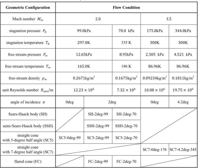
Table 1: Summary of flow conditions and case notation.

Geometric Configuration Flow Condition

Mach number �_∞ 2.0 3.5

stagnation pressure �₀ 99.0kPa 70.0 kPa 175.8kPa 344.8kPa

stagnation temperature �₀ 297.0K 335 K 300K 300K

free-stream pressure �_∞ 12.65kPa 8.95kPa 2.305 kPa 4.521 kPa

free-stream temperature �_∞ 165.0K 186 K 86.96K 86.96K

free-stream density �_∞ 0.2671kg/m3 0.1675kg/m3 0.09234kg/m3 0.1811kg/m3

unit Reynolds number �unit/m 12.23 × 106 7.32 × 106 10.08 × 106 19.75 × 106

angle of incidence � 0deg 2deg 0deg 4.2deg

Sears-Haack body (SH) SH-2deg-99 SH-2deg-70

semi-Sears-Haack body (SSH) SSH-2deg-99 SSH-2deg-70

straight cone

with 5-degree half angle (SC5) SC5-0deg-99 SC5-2deg-99 SC5-2deg-70

straight cone

with 7-degree half angle (SC7) SC7-0deg-176 SC7-4.2deg-345

flared cone (FC) FC-2deg-99 FC-2deg-70

( > 0) , > 0 ( = 0)

(9)

The semi-Sears-Haack body and flared cone configurations were originally designed at JAXA for investigating the influence of pressure gradient on the flow characteristics near the leeward symmetry plane [57].

Table 1 provides the summary of studied cases as well as introducing a composite notation that combines the information about the shape, angle-of-incidence, and stagnation pressure. For example, the case SC5-0deg-99 from Table 1 refers to the straight cone with 5-degree half angle SC at 0-degree incidence and a stagnation pressure of 99 kPa.

The values of stagnation pressure correspond to the experimental conditions, which are conducted by JAXA. The quantities �_∞,�₀,�_∞, and ��unitdenote the Mach number, stagnation pressure,

(10)

3 Summary of Mean Flow Computations

The results of mean flow computations, which were conducted at JAXA and NASA, are compared

with each other. Then, it is confirmed that those are in fairly good agreement with each other. Even

though, there were observed slight differences due to thermal condition, numerical grid and

computational solver. The difference due to the thermal condition is obvious but reasonable, and the

other differences are very small. Moreover, the JAXA grid is confirmed to be sufficient in order to

apply to the linear stability analysis, though the JAXA grid is coarser than the NASA grid.

The investigation of mean flow computations [1-4] is summarized below.

3.1 Computational Methodologies

The laminar basic state at each condition was obtained using numerical solutions to the

compressible Navier-Stokes equations. Due to the long duration of the tests, the test model reaches

thermal equilibrium with the surrounding flow and, hence, the thermal boundary condition at the

model surface corresponds to an adiabatic wall. On the other hand, an isothermal boundary condition

is more appropriate for the short duration tests corresponding to a higher stagnation pressure (�₀ =

99 kPa) in the FWT (the 0.6m×0.6m High Speed Wind Tunnel at Fuji Heavy Industries in Japan).

For the FWT test conditions, the estimated recovery temperature (based on a recovery factor of 0.85)

is 277 K. Thus, the isothermal model temperature of �w = 300 K used for the mean flow

computations corresponds to �w⁄�ad≈1.08.

Two different flow solvers were used for this purpose and extensive comparisons were made

between the respective solutions to ensure that the computed mean flow solutions were independent

of the code. Computations with adiabatic thermal wall boundary conditions were performed using

the 3D, multi-block, structured-grid flow solver UPACS [61], which was developed at JAXA.

Independent computations for the same test conditions were performed at NASA using an analogous

3D, multi-block, structured-grid flow solver, VULCAN [62] that was developed at the NASA

Langley Research Center. Additional computations were done with the VULCAN code to compute

the basic state solutions corresponding to the isothermal wall boundary condition (�w = 300 K).

The computational grids were also independently generated based on knowledge and experience.

The UPACS based computations at JAXA were based on a typical grid size of 120 points in the axial

direction, 150 points in the surface normal direction, and more than 193 points in the azimuthal (i.e.,

circumferential) direction. On the other hand, computations at NASA were based on a typical grid

size of 610 points in the axial direction, 353 points in the surface normal direction, and more than

257 points in the azimuthal direction. The wall-normal grid distribution was similar for both flow

solvers. The nose radius of each axisymmetric configuration was assumed to be zero for the

UPACS computations, whereas the VULCAN computations used a nonzero but tiny nose radius (approximately 4 μm) that was resolved with approximately 65 axial points in the nose region. The number of points in the JAXA computational grid is much less. However, the result showed that the

(11)

3.2 Surface Pressure Distributions and Mean Velocity Profiles

Figures 2(a) through 2(g) display the surface pressure distributions for each body shape and angle

of incidence that were obtained at adiabatic thermal wall boundary conditions by use of UPACS.

Regardless of the body shape, a positive azimuthal pressure gradient was observed at any fixed

axial station at nonzero angle of incidence cases. The azimuthal pressure gradient drives a

circumferential flow from the windward to the leeward side and, hence, causes the boundary layer

flow to become fully three-dimensional. On the other hand, the pressure gradient in the axial

direction varies with the body shape. As alluded to previously, it is favorable along the SH and SSH

body shapes, but almost zero for the SC shapes and adverse for the FC. The favorable pressure

gradient along the length of the SSH body is weaker in comparison with that along the SH body. In

comparison with two straight cones, it was found that the pressure distribution of SC7-0deg-176 case

is qualitatively almost the same as that of the SC5-0deg-99 case, as expected by linear theory for

slender bodies. However, the azimuthal pressure gradient of the SC7-4.2deg-345 case is much larger

than that of the SC5-2deg-99 case.

The axial development of the mean velocity profiles along a generatrix at zero-degrees angle of

incidence, i.e., SC5-0deg-99 and SC7-0deg-176 cases, are virtually self-similar (Fig. 3(a) and Fig.

3(b)). On the other hand, the leeward plane profiles in the SH-2deg-99 case continue to develop in

the axial direction and are not self-similar. The variation in velocity profiles over a similar range of

locations becomes stronger as the magnitude of the favorable pressure gradient in the axial direction

is reduced from the SH body shape (Fig. 3(c)) to the SSH body shape (Fig. 3(d)).

(a) SC5-0deg-99 (a) SC5-0deg-99

(b) SC7-0deg-176 (b) SC7-0deg-176

Figure 2. Surface pressure distribution [1-4].

Figure 3. Mean velocity profiles along the leeward ray [1-4].

(a) SC5-0deg-99 (a) SC5-0deg-99

(b) SC7-0deg-176 (b) SC7-0deg-176

(12)

As shown in Fig. 3, the existence of inflection is even visually obvious in the case of velocity profiles along the leeward ray of the SC5-2deg-99 configuration (Fig. 3(e)). The characteristics are stronger for SC7-4.2deg-345 (Fig. 3(g)) case. And the inflection becomes also stronger when the axial pressure gradient becomes negative (case FC-2deg-99 in Fig. 3(f)). The lift-up effect increases as the axial location moves downstream.

The velocity profiles on the sides and along the windward ray are compared with that along the leeward ray for SC5-2deg-99 case (Fig. 4). The profiles along the windward ray are virtually self-similar as seen from the collapse. On the other hand, it is confirmed that the existence of inflection is even visually obvious in the case of velocity profiles along the leeward ray.

(c) SH-2deg-99 (c) SH-2deg-99

(d) SSH-2deg-99 (d) SSH-2deg-99

(e) SC5-2deg-99 (e) SC5-2deg-99

(f) FC-2deg-99 (f) FC-2deg-99

(g) SC7-4.2deg-345 (g) SC7-4.2deg-345

(completed)

(completed) 0.06

0.00 CpCp

(c) SH-2deg-99 (c) SH-2deg-99

(d) SSH-2deg-99 (d) SSH-2deg-99

(e) SC5-2deg-99 (e) SC5-2deg-99

(f) FC-2deg-99 (f) FC-2deg-99

(g) SC7-4.2deg-345 (g) SC7-4.2deg-345

(completed)

(completed) 0.06

(13)

(14)

�

�0

� 4 Methodologies and Results of Stability Analysis

The laminar mean flows described in the previous section were used as basic states for linear stability analysis to understand the measured transition characteristics near the leeward ray. Computations were performed using the LSTAB [55] code developed at JAXA and the LASTRAC [63] code developed at the NASA Langley Research Center. The growth rates were integrated along selected trajectories along the cone surface to enable a comparison between predicted N-factors (i.e., logarithmic amplification ratios) for unstable disturbances with the observed transition fronts. A selected set of results based on the eN methodology is described below.

4.1 Maximum Growth Envelope Method

The maximum growth envelope method correlates the transition location with the logarithmic amplification ratio (i.e., �-factor) based on the most amplified fixed frequency disturbance. For each frequency, the �-factor distribution over the body surface is determined by integrating the maximum growth rate over all azimuthal wave numbers at each point along a selected set of trajectories. In this paper, these trajectories are taken to be streamlines near the edge of the boundary layer.

4.2 Mode Tracking Method

An alternative to the maximum growth envelope method for �-factor correlations is the mode tracking method. Rather than maximizing the local growth rate over all disturbance wave numbers at a given frequency, the mode tracking method uses the maximum growth envelope of several �-factor curves, each of which corresponds to a nominally fixed disturbance entity in the form of a specified set of frequency-azimuthal wave number (i.e., (�,�) a combination (of specific disturbance modes). Stability computations using the mode tracking approach were performed using the LASTRAC code.

4.3 Results of the Maximum Growth Envelope Method

The growth of a disturbance was traced along two typical stream lines on the SC5-2deg-99 case (Fig. 5). The first stream line (abbreviated as #1 in the following) is that along the leeward symmetry plane. And the second one (abbreviated as #2 in the following) along the side line (a generatrix at�= 90 deg) at � ≈0.2 m.

(15)

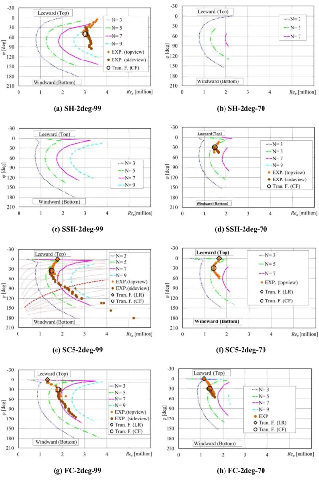
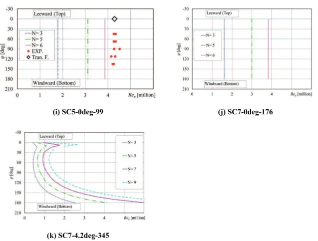
�-factor contours corresponding to LSTAB computations based on the UPACS mean flow solutions for 2-degrees angle of incidence and both values of stagnation pressure in Table 1 (�₀ = 99 kPa and �₀ = 70 kPa cases) were included in Figs. 6(a) through 6(h). And those for SC5-0deg-99, SC7-0deg-176 and SC7-4.2deg-345 cases are also shown in Figs. 6(i), 6(j) and 6(k). As expected, an azimuthally invariant transition front is predicted in the SC5-0deg-99 case and SC7-0deg-176 cases.

�-factor contours for the SH body at nonzero angle of incidence predict a later transition location along the leeward symmetry plane than the neighboring azimuthal locations (Figs. 6(a) and 6(b)). In contrast, computations for the other 4 body shapes (Figs. 6(b) through 6(h) and 6(k)) predict a 3-lobed transition front including a center lobe that is indicative of an earlier transition location along the leeward ray in comparison with the adjacent azimuthal locations. The center lobe moves progressively farther upstream as the axial pressure gradient changes from mildly favorable (SSH) to nearly zero (SC) to adverse (FC). This upstream movement of transition location along the leeward ray is attributed to the higher amplification rates associated with increasingly thicker, and highly inflectional velocity profiles along the leeward symmetry plane (Fig. 3).

(a) Illustration of streamlines on the model in

the SC5-0deg-99 case.

(b) Growth rate predicted along the stream

line #2.

(c) Growth rate predicted along the stream

line #1.

(d) Growth rate predicted along each stream

lines.

Figure 5. Growth rate for the SC5-0deg-99 case. 0 5 10 15 20 25 30 35 40 45

0 0.1 0.2 0.3 0.4

N x[m] 5.0KHz 10.0KHz 15.0KHz 20.0KHz 25.0KHz 30.0KHz 35.0KHz 40.0KHz 45.0KHz 50.0KHz Envelope 0 5 10 15 20 25 30 35 40 45

0 0.1 0.2 0.3 0.4

N

x[m]

5.0KHz 10.0KHz 15.0KHz 20.0KHz 25.0KHz 30.0KHz 35.0KHz 40.0KHz 45.0KHz 50.0KHz Envelope 0 5 10 15 20 25 30 35 40 45

0 0.1 0.2 0.3 0.4

N

x[m]

Stream Line #1

Stream Line #2 �

�0

�

(a) Illustration of streamlines on the model in

the SC5-0deg-99 case.

(16)

�

� �

�

(a) SH-2deg-99 (b) SH-2deg-70

(c) SSH-2deg-99 (d) SSH-2deg-70

(e) SC5-2deg-99 (f) SC5-2deg-70

(g) FC-2deg-99 (h) FC-2deg-70

(17)

(i) SC5-0deg-99 (j) SC7-0deg-176

(k) SC7-4.2deg-345

Figure 6. �-factor contours based on maximum growth envelope method with experimental results

(completed).

As shown in Fig. 6(e), the earliest transition in the SC5-2deg-99 case is predicted to occur along the leeward ray (� = 0 degrees) rather than along the adjoining side surface. The integration trajectories used for �-factor calculations in this case are also shown in the same figure. The apex (i.e., most upstream location) of the crossflow dominated transition lobes on the side of the cone was found to be located at approximately � = 60 degrees, in agreement with a previous prediction for the same cone at the same Mach number [54, 55]. The farthest downstream onset of transition is predicted to occur along the windward ray, i.e., at � = 180 degrees and this location is farther downstream than the predicted transition for a zero angle of incidence case (Fig. 6(i)).

The upstream movement of transition location along the leeward ray and the side area were observed for the SC7-4.2deg-345 (Fig. 6(k)) case, compared with the SC5-2deg-99 case (Fig. 6(e)). On the other hand, the transition location along the windward ray moved to the downstream. Those differences are clearly due to differences of the boundary layer profile depending on the Reynolds number, the cone half angle and the angle of incidence.

(18)

φ

●

● ● 4.4 Comparison of Stability Analysis

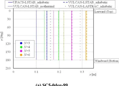
An illustrative comparison of �-factor contours based on the mode tracking method with those obtained with the maximum growth envelope method is shown in Figs. 7. This comparison is made for the SC5-0deg-99, SC7-0deg-176 and SC5-2deg-99 configurations using basic states obtained for an isothermal (�w⁄�ad≈1.08) model surface; however, to illustrate the effect of the thermal

boundary conditions, the results of the maximum growth envelope method for the adiabatic mean flow are also included. For the adiabatic case, results obtained using two different mean flow solvers (VULCAN and UPACS, respectively) but the same stability code (LSTAB) are shown. Because the adiabatic mean flow profiles predicted by VULCAN and UPACS are in close agreement with each other, the resulting stability predictions are also very close to each other.

(19)

(a) SC5-0deg-99

(b) SC7-0deg-176

(c) SC5-2deg-99

Figure 7. Comparison of N-factor contours. -30

0 30 60 90 120 150 180 210

0 0.1 0.2 0.3

φ

[de

g]

x[m] UPACS-LSTAB_adiabatic VULCAN-LSTAB_adiabatic VULCAN-LSTAB_isothermal VULCAN-LASTRAC_isothermal

Windward (Bottom) Leeward (Top)

●N=3

●N=5

●N=7 ●N=9 (a) SC5-0deg-99

(b) SC7-0deg-176

φ

● =3

(20)

have a β

�

All models had a β

The β 5 Method and Results of Experiments

5.1 Wind Tunnel Facilities

The wind tunnel experiments were conducted by JAXA in two different facilities, with the lead author of this paper as the principal investigator. The measurements in each facility provided information about the transition front over the model as well as the static pressure fluctuations in the free stream.

The first facility was the 0.2m×0.2m supersonic wind tunnel (SWT2) at JAXA. [64]. The SWT2 tunnel nozzle has been designed using the method of characteristics and the contraction ratio to the cross-sectional area of the test section is 28.3. A boundary layer suction device is mounted at the contraction in order to provide a low disturbance flow. However, it was not used because the device is not effective in stabilizing the wall boundary layer. A total of 4 screens were employed to avoid flow separation and to establish better flow uniformity. The SWT2 is a continuous flow facility that allows independent and continuous variations in both Mach number (1.5 < �_∞ < 2.5) and total pressure (55 kPa < �₀ < 100 kPa). The nominally controlled total flow temperature �₀ equals 335 K, but can be increased if necessary by terminating the supply of the cooling water. For the work described in this paper, the flow conditions for all tests in SWT2 were fixed at �_∞ = 2, �₀= 70 kPa, and �₀ = 335 K. In other words, the test condition of �₀= 99 kPa for the FWT measurements could not be repeated during the measurements in SWT2 because the capacity of the SWT2 cooling system is rather low to allow continuous operation at the fixed nominal temperature of �₀ = 335 K at the flow condition of interest.

The second facility used in the present work was the 0.6m×0.6m High Speed Wind Tunnel at Fuji Heavy Industries in Japan, which is an in-draft type facility. It will be denoted as FWT in this paper. This wind tunnel nozzle has been also designed using the method of characteristics in conjunction with a correction for boundary layer displacement. A total of 3 screens were employed. The freestream Mach number in FWT can be varied in steps, and was maintained at �_∞= 2 for the experiments reported herein. The total pressure �₀ and total temperature �₀ are almost atmospheric but cannot be prescribed. Therefore, the �₀ and �₀ values vary from run to run; however, the magnitudes of these variations are small, with the resulting variation in the unit Reynolds number being less than 5% and a dew point temperature of less than 258 K.

For transition measurements, the original schlieren window in both wind tunnels was replaced by a sapphire-glass window to enable the measurement of model surface temperature using an infrared (IR) camera at both facilities.

(21)

denotes the root-mean-square value of the surface pressure fluctuation scaled by the dynamic pressure of the free-stream and was measured using a Kulite pressure transducer mounted on a straight cone model at zero degrees angle of incidence.

The measured static pressure fluctuations were lower than those quoted in Refs. 49 and 64 in spite of the wider frequency bandwidth of the present measurement. The Kulite XCS-062 pressure transducer with a diameter of 1.6 mm has a resonance frequency of 150 kHz and a nominal bandwidth of 0 kHz to 50 kHz. However, because of an uncalibrated amplifier, the net estimated bandwidth of the unsteady pressure measurements is limited to the frequency range of 0 kHz to 30 kHz. The cause for this discrepancy from the earlier measurements has not been determined. The static pressure fluctuations in the FWT are comparable to those measured in flight at similar Mach numbers; however, the level of vortical fluctuations and their impact on transition in these facilities remains unknown.

Given the low amplitudes of free-stream acoustic disturbances, both facilities were deemed acceptable, at least for studying the mechanisms for transition within the boundary layer flow along the leeward symmetry plane. As an additional a posteriori assessment of the tunnel disturbance environment, the transition Reynolds numbers for axisymmetric flow past a straight cone in SWT2 and FWT were compared with those in other conventional and low disturbance (i.e., quiet) wind tunnel facilities as well as those measured in a flight experiment. This comparison indicated that the transition behavior in SWT2 and FWT is effectively similar to that in other conventional wind tunnels in spite of the lower levels of free-stream pressure fluctuations in these two facilities. This finding also suggests that the nonacoustic disturbance environment in these facilities (which has not been measured) is likely to have a significant influence on the transition process, but also that the overall flow quality is comparable to that in other conventional tunnels.

5.2 Test Models

(22)

μ μ

×

� �

� ��_� �� _√� ∫ � � −� �_�−� 3 2⁄ ��

�

0 �

� � � � � �

� �

� �� 2

�

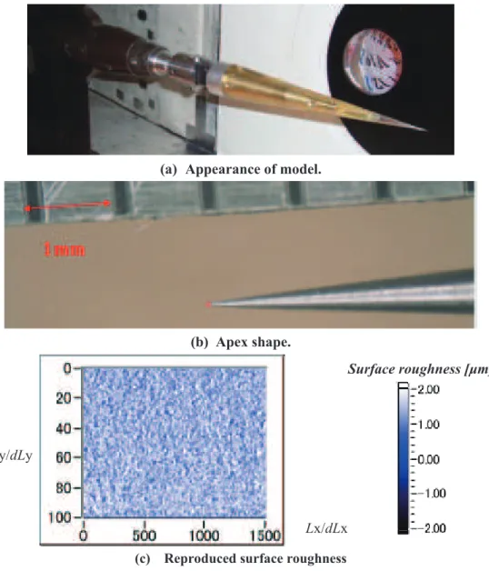
(a) Appearance of model.

(b) Apex shape.

(c) Reproduced surface roughness

Figure 8. Experimental model of SC5 (� = 0.3 m).

To measure the surface pressure fluctuation ��RMS, a Kulite sensor was flush-mounted. The axial

locations of the transducers are different for each model. A total of 4 sensors are mounted on the

straight cone model of � = 0.7 m, all of which are located downstream of � = 450 mm. On the

straight cone model of � = 0.3 m, however, two sensors are mounted on opposite sides of the model

at � = 150 mm (� =90 deg) and � = 250 mm (� = -90 deg), respectively. A single sensor was

mounted at � = 170 mm and � = 180 deg. on each of the FC, SH, and SSH models. Since the

azimuthal locations are different for each test, those are described for each result.

The apex shape was examined through micrographs and was found to have significant azimuthal

variations. The apex diameter is defined as the diameter of a circular fit to the apex shape, averaged

over photographs taken from four different directions. The apex diameter determined in this manner

was found to be different for each model, with the overall range being 41 μm to 260 μm (Fig. 8 (b)).

The nonzero apex diameter is likely to influence the stability and transition processes, especially on

models with a larger nose diameter. However, it was not possible to model these effects during the

computations performed in this study. Ly/dLy

Lx/dLx

(23)

Due care was taken to minimize any surface height discontinuities at the juncture between the

nose and the main part of cone. The juncture was finished following the assembly of the two parts.

Therefore, resulting discontinuities over the actual test article are sufficiently small, such that there is

no difference between the tactile impressions on either side. Hence, the magnitude of juncture

discontinuities is estimated to be nearly the same as that of the surface roughness, which was

estimated by reproducing the roughness pattern on small samples of dental resin (Pattern Resin

1-1PKG). The resin was hardened together with a paper backing that could be easily peeled off with

the help of a hole at the center of the paper. The reproduced roughness on the resin sample was

measured with a laser displacement sensor (LT-8010; Keyence). The roughness amplitudes

(measured as arithmetic mean of roughness heights) for all four models were nearly the same,

approximately in the range of 0.6 μm ~ 0.7 μm (Fig. 8 (c)).

The effects of azimuthal variations near the cone apex and the surface roughness on either the

mean flow or the disturbance evolution within the downstream region are not addressed in this paper.

5.3 Instrumentation and Measurement Methodologies

Since the rate of heat transfer reflects the transport properties of the boundary layer flow, the

transition front can be inferred as the locus of points associated with a rapid axial gradient in surface

heat transfer. The surface temperature distribution was measured using an infrared camera

(TVS-8502, Nippon Avionics Co. Ltd.). This camera provided 256×236 pixel images with less than

0.025 K resolution at the rate of 30 Hz. The corresponding spatial resolution depends on the test case,

and is from about 0.16 mm to about 1 mm. This data was subsequently converted to a surface heat

flux distribution under the assumption of semi-infinite, one-dimensional thermal conduction through

a uniform medium with temperature invariant thermal properties. The heat transfer rate �was a

function of time� has been estimated via the following equation: [65]

�w=�

��

� �

�(�)

√� +∫

�(�)−�(�)

(�−�)3 2⁄ ��

�

0 �

(5)

where �(�) denotes the surface temperature at time �, and �, � and � denote the density, the

specific heat and the thermal conductivity of the material, respectively. To reduce high frequency

noise compared with the period of flow change (typically 60 seconds for SWT2 tests and 10 seconds

for FWT tests),�(�) was approximated by a moving average over a time interval of 5 seconds for

SWT2 tests and 1 second for FWT tests, where the averaging intervals are approximately one order

of magnitude smaller than the corresponding period of interest. Because of the relatively low thermal

diffusivity of the insulative material of the model, the Fourier number (�=��/(��2)) based on the thickness of the model (i.e., the local model radius �) remained less than 0.04 over the duration of

the IR measurement. It suggests the length scale of the lateral thermal diffusion corresponds to a

Fourier number of 1. The low Fourier number implies not only that the penetration depth through the

IR measurement is sufficiently shallow to support the assumption of semi-infinite model thickness

(24)

�

� �

at φ = 180 deg. on each of the FC, S

�0 �0

�0

� �0

� thermal diffusion is small compared with the radius of the model. For the tests conducted in FWT,

the initial surface temperature distribution can be reasonably assumed to be uniform. However, because of the long duration of the tests conducted in the closed circuit wind tunnel SWT2, the temperature distribution at the model surface had nearly reached an equilibrium at the start of the IR measurement and, therefore, the surface heat flux was very small. To obtain a measurable heat flux, a small but sudden, i.e., step-like change, was applied to the SWT2 stagnation temperature (∆�₀≈ 5 K) after reaching the equilibrium temperature distribution for �₀≈335 K. This change in stagnation temperature occurred during a time interval of less than 100 seconds. The 5-degree variation in stagnation temperature is negligible from the standpoint of comparison with the numerical prediction, since it corresponds to a unit Reynolds number variation of just 2%. The measured changes in surface temperature in response to the change in �₀were used in conjunction with Eq. 5 to estimate the heat transfer rates during the SWT2 tests. The initial temperature in this case was obtained from the measured distribution of equilibrium temperature before the step-like change in stagnation temperature was applied. An analogous technique for IR-based transition measurements was used during a recent flight experiment involving crossflow transition at a low subsonic Mach number. The heat transfer distributions inferred via the procedure outlined above are shown in Fig. 9, where the transition front is clearly marked by a sharp, negative axial gradient in the images corresponding to the measurements in FWT and by a sharp positive gradient for the images acquired in the SWT2. The reason behind the opposite gradients in heat transfer distributions in the two facilities is clarified in subsection 5.4 below. Such opposite gradients can be reconciled using a comparison based on the Stanton number distribution, which yields similar trends in both facilities as expected. However, deducing the Stanton number from the heat flux requires the knowledge of stagnation temperature corresponding to each IR image and, unfortunately, the stagnation temperature measurement was not synchronized with the IR measurement. The resulting uncertainty in the stagnation temperature prevents a comparison between the measured heat flux and the CFD results.

(25)

of 1.6 mm. The acquired signal was analyzed using a 16-bit multi-functional digital FFT analyzer (CF-5210; ONO-SOKKI).

5.4 Pattern of Heat Transfer Distribution

Heat transfer maps for the test conditions of interest are shown in Figs. 9(a) through 9(h). All figures were observation from a top view perspective. However, the centerline of the images is not along the leeward ray of the model due to the physical limitations of the camera installation in order to avoid the reflection of the cooling system of the IR-camera itself. The Kulite sensor on the shorter SC is located downstream of the � = 450 mm location, i.e., beyond the axial region included in the IR image from Fig. 9(e). On the SC5 model, the upstream sensor was located at � = 90 deg. and the downstream sensor was at � = -90 deg. in Fig. 9(f) for the SC5-2deg-70 configuration and located at φ = 180 deg. on each of the FC, SH, and SSH models. The presence of these sensors did not have any influence on the temperature distributions in Figs. 9. Even though the edge of the model is less clear against the background of the surrounding tunnel wall, the latter was retained in order to avoid any artificial manipulations of the acquired image. The yellow arrows in each of these figures indicate the location of an aluminum tape that was used as a fiduciary mark along the rear section of the model. The tape thickness was of the order of tens of micrometers. It was placed significantly farther downstream of the transition location and the edges of the tape were pressed down carefully in order to minimize any upstream influence. Therefore, virtually no influence was observed on the transition location. For example, an asymmetric transition pattern was not observed even when the tape was mounted asymmetrically. To allow an estimation of the cone length captured within each image, a pair of thin black horizontal arrows is used in each figure (with the exception of Fig. 9(c)) to indicate a reference length along the model axis. The absence of this pair of arrows in Fig. 9(c) is due to the low accuracy of the reference aluminum tape in the SSH-2deg-99 case. In this case, the aluminum tape (which was prepared before the experiment) was too far downstream of the transition location and, hence, was not included within the IR image. As a temporary fix, therefore, another tape was used to help determine an approximate location of transition.

It may be noted that the distributions of heat transfer at �₀= 70 kPa and �₀= 99 kPa have opposite signs. The data at �₀= 70 kPa was acquired in SWT2 by terminating the cooling water to apply a step-like change in the stagnation temperature of the flow as mentioned above. As a result, the direction of heat transfer is from the flow to the model surface (i.e., �w> 0). On the other hand,

the model temperature for the �₀= 99 kPa runs in the short duration facility, FWT, is higher than the adiabatic surface temperature and, therefore, the flow cools the model, i.e., �w < 0. Nevertheless, in

(26)

side view images obtained by rotating the cone (which are not shown in this paper) are described in subsection 5.5 below.

For the SH body, transition at �₀= 99 kPa is first seen to occur over the side of the cone, i.e., away from the leeward plane of symmetry (Fig. 9(a)). There is actually a local maximum in the transition location along the leeward ray, so that the overall shape of the transition front on the unrolled surface of the SH body (such that the leeward ray is located along the center) resembles a “W” shape that has been rotated counterclockwise by 90 degrees. Henceforth, this shape will be referred to as the “sideways W” pattern. The upstream transition over the side region is believed to have been caused by crossflow instabilities in that region. The shape of this crossflow transition lobe is analogous to that seen previously during quiet tunnel measurements of a Mach 3.5 delta-wing configuration [43] as well as in the course of conventional facility measurements for a yawed circular cone at Mach 6 [59, 65]. The cause of transition along the leeward ray (where the crossflow velocity is identically zero because of symmetry) is not immediately obvious. It could have been initiated by the amplification of linear instabilities of the laminar flow in its vicinity or induced by turbulent contamination from the adjacent region. Figure 9(b) shows that in the lower Reynolds number case SH-2deg-70, the boundary layer flow remained laminar over the entire body surface. Figures 9(c) and 9(d) reveal that, similar to the SH configuration, the SSH body shape also exhibits the “sideways W” shaped transition pattern, with an earlier transition location away from the leeward ray. The main difference between the transition patterns over the two bodies is that for SSH, transition was observed to occur even in the lower Reynolds number case (Fig. 9(d)).

The higher Reynolds number case SC5-2deg-99 (Fig. 9(e)) for the straight cone configuration indicates a qualitative change from the transition pattern observed for the SH and SSH body shapes. The transition front in this case appears to include an additional, narrow lobe centered on the leeward ray. Since there is no crossflow along the leeward ray, the center lobe (which is still small for the SC5-2deg-99 case, but becomes more prominent for the FC configurations in Figs. 9(g) and 9(h)) is attributed to a different transition mechanism than the crossflow effects underlying the outer two lobes within the transition front. Because the earliest transition location within the center lobe occurs along the leeward ray, one may reasonably assume that the underlying cause of transition is the amplification of instabilities along the leeward ray. It is seen, however, that the transition location along the leeward ray is still significantly farther downstream from the earliest onset of transition within the side region. This may be due to the fact that for � = 2 degrees, the secondary flow leading to the thickening of the leeward symmetry plane boundary layer is still relatively weak at the unit Reynolds number corresponding to this case (SC5-2deg-99).

(27)

(28)

∆�

� �1

� �2 �2 �1

� �1

∆�

angle (φ = 30 deg of

(a) SH-2deg-99 (b) SH-2deg-70

(c) SSH-2deg-99 (d) SSH-2deg-70

(e) SC5-2deg-99 (f) SC5-2deg-70

(g) FC-2deg-99 (h) FC-2deg-70

Figure 9. Heat transfer distributions for test conditions of interest (top

view, approximately centered on the leeward symmetry plane). Figures

in the left-hand-side were obtained in FWT, and those in the

right-hand-side were obtained in SWT2.

-258.2

W/m

2

₀

0 W/m

2

₅₀₀

-258.2

W/m

2

₀

0 W/m2 ₅₀₀

-1000

W/m

2

₀

_W/m

2

₅₀₀

-182.6 W/m

2

₀

_W/m

2

₅₀₀

55mm

15mm ~5mm

10mm

15mm

(29)

5.5 Extraction of Transition Location

The maps of heat transfer from the previous subsection outlined the qualitative nature of transition

patterns over the canonical nose configurations of interest. The present subsection describes

quantitative estimates of the transition front in the relevant cases. The transition location was

extracted from the maps of “temperature difference (∆�)” between two selected instants of time for a

given run. For the short duration tests carried out in FWT, the two selected times correspond,

respectively, to the time �=�₁ when the flow condition was stabilized in FWT and some later

instant �=�₂ (�₂>�₁) when a measurable temperature difference had been established with

respect to � =�₁. The corresponding times for the tests in SWT2 are based on the beginning and the

end of the surface temperature response to the step-like change in stagnation temperature.

Axial variations in ∆� along selected cone generators (corresponding to lines of constant

azimuthal angle along the cone surface) are extracted from the surface maps of ∆� using the

location of an aluminum tape as a reference as mentioned previously. The extraction of a selected

cone generators is explained in detail in Appendix A.

For each curve of this type, the transition region and the laminar and turbulent flow regions

immediately upstream and downstream of the transition region are each approximated by a linear

segment (Fig. 10). The point of intersection between the laminar and transitional segments

corresponds to the onset of transition, whereas the point of intersection between the transitional and

turbulent segments defines the end of transition. The midpoint of the straight line segment

connecting the onset- and end-of-transition locations defines the midpoint of the transition zone. The

midpoint locus is used as the measured transition location in the remainder of this paper. The

extracted transition location is shown in Figure 11.

Figure 10. Sample variation of temperature difference along a line of constant azimuthal angle (φ = 30 deg of FC-2deg-99).

The extracted transition for the 7 cases from Table 1 are shown in Figs. 6(a) and (d)-(i).

-4

-3

-2

-1

0

20

40

60

80

100

120 T

em

p

era

tu

re

d

if

fe

re

n

ce

[d

eg

]

(30)

��

�

�∞

�0

�

� �

�

The uncertainty in experimentally inferred transition locations was estimated to be less than

approximately ±5 mm. This estimate includes the combined effect of the finite resolution of the IR

image, the uncertainty in the identification of transition location from the IR image, and the

uncertainty in the correspondence between the IR-image and the physical location on the model. The

light brown circles in Fig. 6 indicate the transition front based on the top view of the model, whereas

the dark brown circles in Fig. 6 indicate the transition front inferred from the side view of the model,

though the side-view results are not shown in this paper. The opposite side transition location

obtained from the top view is superimposed at the corresponding azimuthal location in the figure.

Since the superimposed data at φ < 0 deg overlap the data at φ > 0 deg, no significant asymmetry

was observed. The transition locations in the side view images (not shown) was acquired

independently, but under the same flow conditions. In order to obtain the side view data, the model

was rotated by 90 degrees. There are clear but modest differences between the transition fronts

inferred from the two views of each model. These differences reflect the uncertainty in mapping the

IR image to surface coordinates. The factors contributing to this uncertainty include: curvature of the

model surface, possible inaccuracy in the location(s) of the aluminum tape used as a fiduciary mark,

and inadequate resolution of the IR images. It may be noted that transition fronts for the SH-2deg-70

and the SSH-2deg-99 cases were not extracted, since transition did not occur for the SH-2deg-70

case. For the SSH-2deg-99 case, the accuracy of the reference aluminum tape was also rather low as

mentioned above. On the other hand, the transition location is not extracted in the leeward ray region

for the SSH-2deg-70 case, since it occurs very far downstream and cannot be extracted from the IR

measurement. The open diamond and circle in Figs. 6(a) and (d)-(h) correspond, respectively, to

transition locations along the leeward ray and the minimum of the crossflow transition lobe on the

side, as described below.

Figure 11. Extracted transition locations (FC-2deg-99).

5.6 Comparison with numerical prediction

Next, two separate scalar measures of the overall transition front are extracted from the results

shown in Figs. 6. These two measures correspond, respectively, to the transition location on the

(31)

of both measures for each of the relevant cases are summarized in Table 2, wherein ��_� denotes the

local Reynolds number based on free-stream velocity and kinematic viscosity at the inferred

transition location. Because of the previously mentioned discrepancies between transition fronts

based on the side and top views, the values of the scalar measures are averaged over the two views

as necessary. The transition locations for the FC-2deg-99 and the FC-2deg-70 configurations are

monotonically increasing functions of the azimuthal angle �from the leeward ray and, hence, the

minimum of the side lobe could not be identified. Therefore, the location at � = 30 degrees is listed

in the Table. The transition front measures extracted in this manner are shown in Figs. 6(a)-(i) by a

large black open diamond and circle, respectively.

The transition Reynolds number of 4.29 million for the straight cone at zero angle of incidence

falls between the range of transition Reynolds numbers observed in previous flight experiments at

Mach 2 and conventional wind tunnel measurements for slightly higher Mach numbers (�_∞= 2.5 to

4.0) but similar values of unit Reynolds number [53, 54]. The fact that the measured transition

Reynolds numbers are considerably lower than those in flight [62] cannot be easily reconciled with

the low values of measured free-stream pressure fluctuations in the SWT2 and the FWT facilities. A

more detailed study of the free-stream disturbance environment may help explain this finding.

The experimentally observed transition front with occurrence of a center lobe in the transition front over the SC and FC bodies and its absence over the SSH body at �₀= 99 kPa is in agreement with the predicted transition fronts. The absence of early transition along the leeward ray is an open question. However, while the measured transition front for the SSH body showed later transition along the leeward ray, the corresponding �-factor contours do predict a local minimum in the transition location along the leeward ray. This discrepancy suggests that the simplistic approach of correlating multiple transition mechanisms using a single N-factor value is not realistic for this flow and that the �-factor value correlating with crossflow induced transition over the side region is sufficiently smaller than the �-factor value correlating with transition due to first mode instability along the leeward ray. Such differences in

(32)

�

� �0

� ��

The numerically predicted �-factor values at the measured transition locations along the leeward ray and the farthest upstream location of the crossflow transition lobe (see Figs. 6) for the various flow configurations are summarized in Table 2. It may be observed that the �-factors at the transition location along the leeward ray are always greater than 13.5 and, hence, are much higher than the �-factor value of 6.2 correlating with measured transition under axisymmetric conditions. Quiet tunnel measurements [51] for axisymmetric flow over a cone indicate N-factor values of 9 to 10. The finding that � = 6.2 under zero angle-of-incidence conditions can be explained by the fact that conventional tunnels yield lower correlating N-factors than quiet tunnels. On the other hand, the increase in �-factor for transition along the leeward ray is much too large to be explained by the fact that the measured transition location is based on the middle of the transition zone rather than with the transition onset location (which is only about 10 percent upstream compared to the midpoint of the transition zone).

One possible reason for the extraordinarily high �-factors for leeward plane transition could be related to potential differences between the computed and actual boundary layer profiles due to a lack of sufficient information concerning the imperfections of the model tip and/or flow quality effects such as flow angularity, etc. However, the high �-factor values are observed for more than one body shape, i.e., two different models with separate nose tips. Furthermore, it is shown in Ref. 2 that analogously high

�-factors are also found for a completely different 5-degree cone model that was used by King [53] during his quiet-tunnel experiments at Mach 3.5. Thus, the effect of nose tip imperfections or flow angularity would appear to be an unlikely explanation for the high �-factors along the leeward plane. An entirely different explanation involves possible shortcomings of the classical stability theory underlying the �-factor correlations from Table 2. Specifically, it is possible that the azimuthal gradients of the basic state, although zero along the leeward ray, become large enough in the immediate vicinity of the leeward symmetry plane to influence the disturbance evolution within the leeward plane. These azimuthal gradients are not accounted for in the classical stability theory. An additional contributing factor could be related to potentially weaker receptivity mechanisms for the leeward flow in comparison with those of the axisymmetric boundary layer, perhaps because of the somewhat higher frequencies of the relevant instability modes and the associated decay in the amplitudes of the free-stream disturbances, which could cause a delay in transition and lead to the higher � factors.

In comparison with the �-factor values along the leeward symmetry plane, the corresponding

(33)

of nose tip, curvature discontinuity, and small scale perturbations in surface geometry) and the potential presence of nonacoustic free-stream disturbances.

While the presence of crossflow plays an important role in influencing the amplification of instability modes in the side region, the role of first mode waves and stationary and traveling modes of crossflow instability cannot be established on the basis of available measurements. Indeed, in spite of decades of research involving transition in 3D, high-speed boundary layer flows, this fundamental difficulty is yet to be overcome. The linear stability results plotted in Figs. 6 show that the N-factor contours in the side region (which are dominated by traveling crossflow instability) indicate rather small variations from one body shape to another. Indeed, for example, the apex of the

N = 9 contour within the side region moves by less than 10 percent across the four body shapes considered in this paper. Although not shown, similar insensitivity to axial pressure gradient was also noted in the N-factor contours for purely stationary crossflow instability. Thus, the most significant effects of axial pressure gradient on boundary layer stability are confined to the vicinity of the leeward plane.

As mentioned above, the precise cause behind transition cannot be established due to the difficulty in making in-depth disturbance measurements. Nonetheless, some limited comparisons could be made between linear stability predictions and the experimental measurements. Surface pressure fluctuations measured using the Kulite sensor can provide potentially useful information concerning boundary layer disturbances at the sensor location [66]. The azimuthal location of the sensor could be varied, allowing one to obtain measurements at multiple values of �.

Table 2: Summary of transition locations.

Shape � [deg]

�0

[kPa]

Transition front along leeward symmetry plane

Apex of transition front within side region

�[m] ��,�� [million]

�- LSTAB

�-

LASTRAC comment �[m]

��,��

[million]

�

[deg]

�-

LSTAB comment

SC 0

99

0.33 4.29 6.2 5.6 extra- polated SH

2

0.24 3.02 50 9.6 - SSH

SC 0.14 1.79 18.4 16.9 - 0.12 1.51 35 5.5 - FC 0.11 1.32 13.5 10.9 - 0.15 1.80 30 6.2 at 30 deg SH

70

SSH 0.21 1.48 30 5.2 -

(34)

33

Figure 12(a) shows the frequency spectra of surface pressure fluctuations for three different values

of � in the case of the SC5-2deg-70 configuration. The spectra for ��= 0 deg and � = 90 deg

reveal high amplitude disturbances within specific frequency bands indicating the presence of

potential instability amplification. The frequencies corresponding to the spectral peaks of surface

pressure fluctuation at the Kulite location are approximately 20 kHz for ��= 0 deg (i.e., the leeward

symmetry plane) and 40 kHz when ��= 90 deg. Recall that, because of the frequency limitations of

the amplifier, the estimated bandwidth of the unsteady pressure measurements is limited to 30 kHz

and, therefore, the peak near 40 kHz provides only a qualitative measure of the underlying

disturbance amplitudes. At this location, the predicted wave angle is very close to 90 deg with

respect to the inviscid flow direction. Therefore, the disturbance is expected to be a traveling

crossflow mode. The spectral peak for ��= 0 deg is broad, but the increase in amplitude near 20

kHz (relative to the background fluctuations away from the peak) is clearly seen for ��= 90 deg.

The reason of the broadness for φ = 0 deg is an open question.

The frequency of the most amplified disturbances as predicted by the stability analysis was

compared with the frequency spectrum of the experimentally observed surface pressure fluctuations.

According to the maximum growth envelope method, the most amplified disturbance at the Kulite

location had a frequency of more than 50 kHz along the leeward ray and about 40 kHz at φ = 90 deg. The predicted frequency agrees reasonably well with the measured spectrum at φ = 90 deg, but is larger than the measured peak frequency along the leeward ray.

(a) Frequency spectra of measured surface pressure fluctuations along leeward ray

(b) Predicted -factors as functions of disturbance frequency

Figure 12 Comparison between frequency spectra of measured surface pressure fluctuations and the -factor predictions as a function of disturbance frequency for the SC5-2deg-70 configuration.

The precise reason for the discrepancy in disturbance frequencies along the leeward ray could not

be determined. However, it might again be related to the various factors that were outlined above in

the context of the large N_{-factor values along the leeward ray. Kulite measurements were also}

obtained along the windward ray, but the disturbance amplitudes in the experiment were too small to

yield an adequate signal-to-noise ratio; hence, those measurements cannot be compared with the

theoretical predictions. 0.001 0.01 0.1 1 10

100 1000 10000 100000

P o w er D en si ty D is tr ib u ti o n [P a 2/H z] Frequency [Hz] �= 0 deg

�= 90 deg

0 2 4 6 8 10 12 14

100 1000 10000 100000

N

Frequency [Hz] α=2 deg, φ=0 deg

(35)

6 Summary

Boundary layer transition on axisymmetric bodies at a nonzero angle of incidence in a supersonic freestream was investigated via experiments and numerical computations as part of joint research between the Japan Aerospace Exploration Agency (JAXA) and the National Aeronautics and Space Administration (NASA).

Transition over four axisymmetric bodies (namely, a Sears-Haack body, a semi-Sears-Haack body, two straight cones and a flared cone) with different streamwise pressure gradients was studied. The experimental measurements included visualization of the transition front via heat transfer distributions inferred from the surface temperature measurements using an IR camera, along with limited measurements of surface pressure fluctuations and mean boundary layer profiles along the leeward symmetry plane. The measurements indicate that the boundary layer transition along the leeward symmetry plane may occur earlier than that along the neighboring azimuthal locations, when the streamwise pressure gradient is zero or adverse. The earlier transition along the leeward ray under adverse axial pressure gradients is consistent with the computational predictions, which indicate increasingly thicker and more strongly inflectional (and correspondingly more unstable) boundary layer profiles along the leeward symmetry plane when the streamwise pressure gradient becomes relatively more adverse. The destabilizing effect of pressure gradient on the boundary layer flow within the leeward symmetry plane is analogous to that in purely two-dimensional (or axisymmetric) boundary layer flows at both subsonic and supersonic Mach numbers [67-72]. However, in the present context, the cause behind this destabilizing effect is entirely different, being related to the three-dimensional dynamics involving an increasing build-up of secondary flow along the leeward symmetry plane under an adverse axial pressure gradient. This secondary flow is also shown to induce a strongly dissimilar behavior of boundary layer profiles along the leeward ray even though the boundary layer development over the rest of the cone is nearly self-similar and the instability amplification characteristics in that region are relatively insensitive to the axial pressure gradient. Under zero-angle-of-incidence conditions, the same conical configurations do not display a similarly dramatic effect of body shape on boundary layer stability as observed along the leeward plane under a nonzero angle of incidence. Computations also confirm the weakened instability of the boundary layer flow along the leeward symmetry plane when the axial pressure gradient is sufficiently favorable. However, additional analysis is necessary to establish whether turbulent contamination from the adjacent region of crossflow dominated transition might play a role during transition along the leeward plane under the favorable pressure gradient.

This paper provides the IR-based global measurements of boundary layer transition over a yawed circular cone in the supersonic regime, albeit with a significant uncertainty in the quantitative data pertaining to transition locations. More important, the profound effect of axial pressure gradient on the transition behavior along the leeward symmetry plane of slender axisymmetric bodies at a nonzero angle of incidence has been demonstrated.

(36)

and the experimentally observed transition fronts for certain cases, as well as indicating rather high

N-factor values for leeward transition even in a conventional facility. These discrepancies indicate the potential sensitivity of boundary layer transition along the leeward symmetry plane to external disturbances and/or to turbulent contamination, and hence underscore the limitations of N-factor correlations for boundary layer flow involving multiple instability mechanisms. The need to perform more detailed measurements of leeward line transition, both in terms of basic state profiles and the boundary layer perturbations, especially in a low disturbance environment, is also highlighted by the present findings. Resolving these discrepancies and addressing the need for more definitive measurements are important topics for follow-on work.

Acknowledgments

The JAXA authors would like to express thank for the advice from Dr. K. Yoshida, Dr. T. Atobe, along with the graduate technical trainees, Mr. A. Nose, Mr. T. Murayama, Mr. K. Fujisaki, Ms. T. Osada from Gakushuin University and Mr. T. Kawai, Ms. A. Tozuka from Aoyama-Gakuin University.

JAXA Repository AIREX: Pressure Gradient Effects on Transition Location over Axisymmetric Bodies at Incidence in Supersonic Flow: Progress Report of JAXANASA Joint Research Project on Supersonic Boundary Layer Transition Part 2

JAXA Research and Development Report

September 2017

Japan Aerospace Exploration Agency

Pressure Gradient Effects on Transition Location over

Axisymmetric Bodies at Incidence in Supersonic Flow

- Progress Report of JAXA-NASA Joint Research Project

on Supersonic Boundary Layer Transition (Part 2)

on Supersonic Boundary Layer Transition (Part 2) -

Contents

Nomenclature

∞

-258.2

W/m

0

0

W/m

500

-258.2

W/m

0

-1000

W/m

0

0

W/m

500

-182.6 W/m

0

0

W/m

500

-4

-3

-2

-1

0

0

20

40

60

80

100

120

T

em

p

era

tu

re

d

if

fe

re

n

ce

[d

eg

]

₀

₅₀₀

₀

₀

₀

_W/m

₅₀₀

₀

₀

_W/m

₅₀₀