NETWORK SCREENING:

(1)

九州大学学術情報リポジトリ

Kyushu University Institutional Repository

ネットワークスクリーニング : 活性化制御ネットワーク同定のための知識ベースの手法

齊藤, 秀

九州大学大学院システム生命科学府

https://doi.org/10.15017/21710

出版情報：Kyushu University, 2011, 博士（システム生命科学）, 論文博士バージョン：

権利関係：

(2)

NETWORK SCREENING:

A KNOWLEDGE-BASED METHOD FOR IDENTIFYING ACTIVE

REGULATORY NETWORKS

齊藤秀

(3)

The global development of resources for omics data enables us to handle the thousands of activities of molecules simultaneously, providing a comprehensive overview of the complicate biological systems. Especially global gene expression profiles by DNA microarray have been extensively measured for a broad range of phenotypes, and several databases consolidate it [1][2]. Accordingly, a lot of methods to analyze the microarray data have been developed regarding preprocessing (e.g. normalization, filtering), clustering, classification and differential analysis. The clustering approaches such as hierarchical clustering [3], K-means [4] and self organization map (SOM) [5]

have successfully applied in the early stage. Now we can use the state of the arts machine learning methods with feature selection [6] such as weighted voting [7], k-nearest neighbor [8], Fisher linear discriminant analysis [9], multilayer neural network [10], support vector machine (SVM) [11] and random forest [12], to predict phenotypes (e.g. disease or normal) from expression signature. In current, the differential analysis is one of promising approach, which enables us to obtain expression signature relating phenotype difference, e.g. authentic statistical test:

parametric t-test, non-parametric Mann-Whitney's U-test and significance analysis of microarrays (SAM) [13]. In above three approaches commonly give us only a gene list as signature, therefore some annotation procedures are required for biological interpretation. However, it is not easy task because of limitation of measurement technology. Since microarray data generally contains several types of noise in terms of individual, biological, experimental level, and there is no longer any information for localization of genes, there is no guarantee that genes having similar profile share similar function as implicit assumption. Recently, several gene set analysis methods were developed to improve ease of interpretation, hypergeometric distribution [14] and gene set enrichment analysis (GSEA) [15]. However, in principle, those methods have limitation for describing complex system behind the data since they neglect relationships among genes. In this situation, development of a novel method considering interactions among molecules (i.e. network) rather than each individual molecular function has become much more important. Therefore, to elucidate networks responsible for the mechanism of the biological systems from measurements for molecules have been important in research area of Systems Biology. Here, we describe belief overview of network based approaches in terms of network inference and knowledge based method.

(7)

5 1.1 Network Inference

Extensive studies have been undertaken in order to infer gene regulatory networks from gene expression data. Several methods have been developed such as Boolean network [16], Bayesian network [17], graphical Gaussian modeling [18], and mutual information-based network [19].

Boolean network is originally introduced by Kauffman [16]. In this framework, each node has one of two discrete states, i.e. on or off, at arbitral time point. The state of a node at time t+1 can be modeled by a Boolean function of k nodes state. Mathematical aspects for Boolean network for gene regulatory network have been reported by Akutsu et al [20], following it, mathematical definition is given as follows.

A Boolean Network G(V,F) consists of a set V={v1,…,vn} of nodes representing genes and a list F=(f1,…,fn) of Boolean functions, where a Boolean function fi(vi1,…,vik) with inputs from specified nodes v_i1,…,v_ik is assigned to each node v_i. For a subset U  V, an expression pattern  of U is a function from U to {0,1}. States of the Boolean Network G(V,F) correspond to expression patterns of V. That is,  represent the states of nodes (genes), where each node is assumed to take either 0 (not-expressed) or 1 (expressed) as its state value. Typically, when the usage is clear from the context, we omit . For example, we write v_i=1 for denoting (vi)=1. In a Boolean network, the expression pattern t+1 at time t+1 is determined by Boolean functions F from the expression pattern  at time t (i.e. t+1(v_i)=f_i(v_i1,…,v_ik)). It is convenient to consider the wiring diagram G’(V’,F’) of a Boolean network G(V,F) (Figure 1.1). For each node vi in V, shch that vi1,…,vik are input nodes to vi in G(V,F). We consider an additional node v’i and construct an edge from v_ij to v’_i for each 1  j  k. Let G’=(V’, F’) the network with nodes v1,…,vn,v’1,…,v’n constructed in this way. Then, the expression pattern of the set {v’1,…,v’n} is determined by v’i=f(vi1,…,vik). That is, the expression of pattern {v1,…,vn} corresponds to one at a time t and the expression pattern of {v’1,…,v’n} corresponds to one at time t+1. Moreover, it is convenient to consider the expression pattern of {v1,…,vn} as the INPUT, and the expression pattern of {v’1,…,v’n} as the OUTPUT.

(8)

6

Figure 1.1 A Boolean network and its wiring diagram.

A network model of three nodes (left), its wiring diagram (middle), and its Boolean function (right) are described.

Boolean network has limitations for treating only time series data, and requiring discretization of continuous gene expression level. Especially in later limitation, inaccurate inferred network due to biological noise is seriously occurred in actual analyses.

Bayesian network is originally proposed by Friedman to build probabilistic model for reasoning under uncertainty [21]. In this framework, joint distribution probability of a directed acyclic graph (DAG) is modeled as a product of the individual node probability density functions conditioning on their parent nodes. One of important research theme for Bayesian network is to develop algorithm for obtaining accurate network structure in reasonable computational time, which have called “structure learning”. Currently, approaches for structure learning are roughly divided into two categories. One is

“score-based method”, which provides a structure by maximizing some scoring function respect to the posterior probability of the structure. As typical scoring function, Bayesian Dirichlet equivalent (BDe) [21] and Bayesian information criterion (BIC) [22]

can be listed. Moreover, as maximization method, several methods such as greedy, K2 [23], Markov chain Monte Carlo [24] have been proposed. Another one is

“constraint-based method”, which provides a structure by checking conditional independency among nodes in the graph. There are several constraint-based methods such as SGS/PC-algorithm [25], CI-algorithm [17]. The score-based methods try to get an optimal structure in terms of likelihood (i.e. goodness-of-fit of the model). On the other hand, the constraint-based method focuses on consistency of conditional independencies in the graph (local Markov property). According to improvement of measurement technology like DNA microarray, Bayesian networks have become a quite popular approach for genetic network inference [26]. Nevertheless a lot of successful

V’1 = V2 V’2 = V1 AND V3 V’3 = NOT V1 G(V,F)

V1

V2 V3

V’1 V’2 V’3

V1 V2 V3

G’(V,’F’)

AND

INPUT OUTPUT

V1 V2 V3 0 0 0 0 0 1 0 1 0 0 1 1 1 0 0 1 0 1 1 1 0 1 1 1

V’1 V’2 V’3 0 0 1 0 0 1 1 0 1 1 0 1 0 0 0 0 1 0 1 0 0 1 1 0

(9)

7

applications of Bayesian network under various biological settings can be enumerated, Bayesian network still have several limitations. One is that Bayesian network accepts only acyclic graphs, i.e., they cannot represent feedback loops in the networks. It is well known that cyclic machinery is common mechanism in various biological functions.

Another is more serious problem, arbitral structure learning in Bayesian network is an NP-hard problem, which means that we are allowed to use only heuristic strategies for finding approximate solutions. But yet, Bayesian network has certain worth in terms of its handiness and ease of interpretation. Since proposed method in this thesis is based on Gaussian Network, which is one of Bayesian networks, we are going to describe brief mathematical frameworks in later chapters.

Graphical Gaussian Modeling (GGM) is one of undirected graphical model, which graphically describes a structure of conditional independency among N variables under the N dimension normal distribution with mean vector μ=(μ1,…,μN)^T and positive definite covariance matrix =(σij), where 1 ≤ i, j ≤ N [18]. In this framework, arbitral two variables having an edge that indicate directly (not through another variable) linear relationship can be obtained. The strength of the direct correlation is expressed by the partial correlation matrix Pij|rest, which describes the correlation between arbitral two variables i and j conditioned on all other variables as follows.

jj ii

ij rest

Pij



 

| (1)

Where ωij is the ij-th element of the precision matrix Ω = Σ^-1. Note that GGM cannot be applied when N < G, because the sample covariance matrix is singular in this case, then the partial correlation cannot be calculated. In addition, highly linear dependences among the variables are frequently occurred in given dataset, especially biological data, which invoke the problem of multicollinearity. Actually, in the gene network inference form microarray, these problems are serious since there are relatively few samples (at most hundreds) and a lot of genes (at least ten thousands) in general. Therefore, to avoid these dimensionality problems, GGM has been applied to only restricted among small number of genes [27][28][29] or among a small number of clusters of genes [30][31].

To overcome this situation, several methods have been developed such as Moore-Penrose pseudo inverse [32], L1 lasso regularization [33], which enable us to obtain sparse large gene network from small number of microarrays.

Mutual information (MI) is originally proposed by Shannon [34] in information

(10)

8

theory, and one of important metric to measure distance between two random variables.

Recently, a gene regulatory network inference algorithm based on MI, named ARACNe [19], was developed and then, several successful applications have been published in important research fields [35]. Its algorithm is simple. First of all, MI with Gaussian kernel between two variables with M samples is estimated by following equation.

   

   





i i i

i f x f y

y x f y M

x

I ,

1 log

, (2)

Where joint probability distribution f is approximated as follows:

 

¹ ²



¹



^,

^

i^, i

^

^, i

i z x y

z z h G M h

z

f ^ 



^ ^ ^ ^ ^ ⁽³⁾

where G(…) is the bivariate standard normal density.

Authors proposed an algorithm for searching consistent edges, named “Data Processing Inequality” (DPI), which extracts edges with following property if the interaction network is g₁  … g2  … g3.



g₁,g₃



min



I



g₁,g₂

 

;I g₂,g₃

 

I  (4)

This procedure is equivalent to check conditionally independence in local network structure. As advantages of MI based approach, authors claimed that their method can reconstruct asymptotically accurate networks having loop topology, and outperform other methods such as simple relevance networks and Bayesian networks [36].

As mentioned above, since inferred networks are expected to detect particular interactions regarding biological phenomena in theory, those methods have been widely used for practical problems. Nevertheless, it is often difficult to interpret for biologists, because reliability of inferred relationships in the networks is frequently uncertain. As reasons for that, two points can be listed: the number of measured points is far less than the number of genes, and the biological and measurement noise strongly affect inference precision. Consequently, in order to obtain biologically meaningful results from the inferred interactions, carefully validations by biological experiment with a lot of effort are required.

(11)

9 1.2 Knowledge-based Method

On the other hand, several methods to detect consistent networks responding measured data from pre-defined known networks were proposed [37][38]. Detected networks by those methods are relativity easy to understand, since those are based on the accumulation of much biological knowledge. Therefore, recently, several databases of experimentally validated interactions have been developed extensively [39][40][41].

Such a vast amount of collected interactions is related to various biological phenomena in the various species, organs, and environments. Unfortunately, because of its volume, those cannot be understood intuitively, it is necessary to focus on contents regarding the research purpose, but it is not trivial. An assumption that whole interactions in the database relate a particular biological phenomenon is unacceptable. Thus, to develop a novel method detecting specific networks responsible for the biological phenomena from a huge amount of known networks is essential for comprehensive understanding biological machinery. Although the approach based on known networks is attractive, it has several pitfalls in practice. First, all interactions in the database should not be treated equally, because those are ensemble of results that discovered in different circumstances, by different researchers, and for different objects. Moreover, we cannot obtain new findings for structural information from identified known networks. In terms of these points, known network approach and inference network approach are trade off. One solution for this is use of chromatin immunoprecipitation (ChIP) data. The ChIP technologies (e.g. ChIP-on-Chip, ChIP sequencing) allow us to measure ability that a particular protein binds to DNA [42][43]. By using binding networks of a transcription factor based on the ChIP data instead of already-known networks, we can evaluate a specific network relating to phenotype (this is neither knowledge-base nor statistical inference). However, it can be applicable to limited number of target transcription factors since the experimental cost cannot be ignored in current situation, and no effective method by combination of ChIP and gene expression data has been developed.

1.3 Motivation

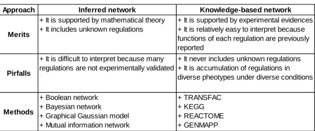
Table 1.1 summarizes above discussion regarding merits and pitfalls for mathematical inference-based and knowledge-based approaches.

(12)

10

Table 1.1 Merits and pitfalls for inference and knowledge-based approaches

A method we will propose in this thesis is based on the knowledge-based approach, because it has advantage in terms of ease of biological interpretation. However, the knowledge-based approach also has a critical pitfall due to diversity of their origins, which come from large variety of phenotypes under various conditions. Therefore, what is required to overcome the pitfall is to develop a screening method for active regulations responsible for the phenotype from vast amount of known regulations. This is a motivation in this thesis.

1.4 Thesis Overview

In the next chapter, we give a framework of our method. At first, we define two statistical methods to evaluate the goodness-of-fit between a network and a measured data. Then to demonstrate our method, we show an example using a toy model and an artificially generated data. Moreover, we evaluate robustness of our method in terms of data dimension, noise level, noise distribution and network topology. Secondly, we propose a concept, which we have named "network screening", which select the specific network candidates that are consistent with the data measured under a particular condition, from an ensemble of known networks. Furthermore, the possible application to real data of our method and the network screening is shown by using the measurement data of Escherichia coli. In Chapter 3, we show three applications of the network screening. First one is application of the network screening to type 2 diabetes data with knowledge base generic transcriptional networks to identify macroscopic functional characteristics of diabetes progression. Secondly, we show effectiveness of the network screening for ChIP data by applying our method to transcription networks for Yamanaka factors based on ChIP data in iPS cells. Finally, we show that the network

Approach Inferred network Knowledge-based network

Merits

+ It is supported by mathematical theory + It includes unknown regulations

+ It is supported by experimental evidences + It is relatively easy to interpret because functions of each regulation are previously reported

Pirfalls

+ It is difficult to interpret because many regulations are not experimentally validated

+ It never includes unknown regulations + It is accumulation of regulations in diverse pheotypes under diverse conditions

Methods

+ Boolean network + Bayesian network

+ Graphical Gaussian model + Mutual information network

+ TRANSFAC + KEGG + REACTOME + GENMAPP

(13)

11

screening is useful for identifying master regulators responsible for glioblastoma. In Chapter 4, as conclusion, the main results of this thesis are summarized and an outlook to future work is given.

2 Methods

Here, we mainly describe a method to evaluate consistency of a given network structure and a data [38]. In this method, a given network is described as a causal graph, and then the causal graph is parameterized on a graphical model, as a result, log-likelihood of the graphical model is calculated. In order to evaluate statistical significance for the log-likelihood, a new statistical measure, which we have named “Graph Consistency Probability” (GCP), is estimated on the log-likelihood distribution of randomly generated graphs. Figure 2.1 summarizes overview of proposed method.

Figure 2.1 Overview of proposed method.

The likelihood (l(G0)) for a “Tested Graph” (G0) from the “Measure Data” is estimated, according to the known procedure for estimating the consistency of the graph with the measured data in Gaussian Graph, in the upper side. The original procedure for translating the likelihood to the probability is described in the lower side.

In the following sections, we are going to describe details for each step.

(14)

12 2.1 Causal Graph

Causal graph is known as a model that graphically shows causal relationships among variables [17].

Figure 2.2 A simple causal graph.

A model with three variables (X1, X2, and X3) is described.

Figure 2.2 shows a causal graph described as a directed acyclic graph (DAG), which denote that measurements of variable X3 depend on the condition of X1 and X2. As a graphical model corresponding the DAG, probability density function of the graph G can be described by product of conditional probability density function with node Xi and its parent nodes pa{Xi}.

        



 ⁿ^v

i

i i

n f X pa X

X X

f G f

1

1,, | (5)

Where pa{Xi} is the set of variables corresponding to the parents of Xi in the graph G.

On the assumption that the probability variable Xi is subjected to a multiple normal distribution, which named “Gaussian Network” (GN) [44], each conditional function in equation (5) is obtained by linear regression of the constituent nodes measured at m points as follows.

 

 















 



 

 

 

 

m

k

n

j

jk ij ik

i i i

i

x x

X pa X f

1

2

1

2 2 2

exp 1 2

| 1 

  (6)

Where xik is the observed value of Xi, at the k-th point, and ni is the number of variables corresponding to the parents of Xi.

(15)

13

2.2 Quantification of Consistency between Model and Data

To quantify goodness-of-fit of the model, the logarithm of the likelihood of the equation (5) is calculated for the measured data as follows.

 

  _ _ _  



     











 











 





 ^v ⁿ^v ⁱ ⁱ

i n

j

i m

k

n

j

kj ij ik

i n

i

i pa X x x

X f G

l

1 1

2 1

2

1 2

1

0 1 ln2

2

| 1 ln

)

(  

 (7)

Thus, the GN allows us to quantify a given network into the corresponding numerical value from the measured data, according to the network structure. Relatively large log-likelihood indicates that the model is acceptable in context of the GN. Note that the calculation of likelihood itself requires no assumptions on the relationships between variables. Indeed, the likelihood can be calculated in the case of non-linear regressions like arbitrary spline regression.

Now, we can obtain the log-likelihood as a consistency measure, then how can we evaluate whether the log likelihood is statistically significantly high? In the following sections, we will describe statistical methods to evaluate significance for the log-likelihood due to graph structure. Generally, it is unknown that the distribution for log-likelihood of a graphical model that depends on graph structure. Therefore, we propose an affinity metric of a graph and a data, named "Graph Consistency Probability" (GCP) [38], which can be calculated by using sampling techniques. In the following two sections, we will describe two methods by generalized extreme value distribution and by nonparametric statistics.

2.3 Evaluation Method using Generalized Extreme Distribution

We can estimate the probability of l(G0) in equation (7) by using the generalized extreme value distribution (GEV) [45] on assumption that l(G0) is extremely high against random structure graphs. First, the log-likelihoods of an ensemble of n random networks generated according to the GN are calculated, and then the maximum log-likelihood is selected from them. The above procedure is iterated m times.

(16)

14

     

 

     

 

     



n^m



m m m

n n

G l G l G l Max l

,..., ,

2 1 m ax

2 2

2 2 1 2

m ax

1 1

2 1 1 1

m ax







(8)

The distribution of the maximum values by m iterations is expected asymptotically to be a generalized extreme value distribution, i.e.,















 



 



 



 







 



 

1 max

max) exp 1

( l

l

G (9)

defined on the set,







 



 



 

 0

1

: ^max

max 

 ^l 

l (10)

where the parameters satisfy -∞ < μ < ∞, σ > 0, and -∞ < ξ < ∞. The model has three parameters: μ, σ, and ξ are a location parameter, a scale parameter, and a shape parameter, respectively. Maximization of the log-likelihood of equation (9) with respect to the parameter vector (μ, σ, ξ) leads to the maximum likelihood estimate for any given dataset, using nonlinear optimization technique. We used the R extRemes package [46]

to fit the data to the GEV distribution by Nelder-Mead method. Note that the standard likelihood ratio test cannot be applied straightforwardly to present case. This is because the density function of the population and the degrees of freedom in the likelihood ratio test are unknown when maximizing the likelihoods of the randomly generated graphs.

In the present method, the GEV distribution of the maximum values of log-likelihoods in the blocks of generated graphs is adopted analogically, instead of the maximum likelihood in the likelihood ratio test. The utilization of the GEV distribution requires the model fitting to the data, but allows us to set the significance probability arbitrarily, as usual in statistical tests. If the goodness-of-fit of the maximum values from the generated graphs is ascertained, then the occurrence probability of a given graph, named

(17)

15

the GCP, can be directly estimated by corresponding the l(G0) in equation (7) to the probability density function of GEV obtained in equation (9).

 

_max

)

( max

0

) ( )

(G G l dl

l

P ^



l^G ⁽¹¹⁾

2.4 Evaluation Method using Nonparametric Statistic

There are two pitfalls in calculation of the GCP by the GEV method proposed in the previous section. One is regarding an empirical parameter; the parameter of sampling period n in the GEV method is only determined empirically. Another is assumption about distribution form of log-likelihood. In the sampling step of randomized graphs, it is frequently occurred to skew a shape of the distribution due to topological restriction of the graphs. Therefore, we propose a method that does not require the empirical parameters (i.e. only sampling times required), does not depend on the distribution form, as follows.

r s

N

GCP N (12)

Where, Nr is total number of randomly generated graphs, Ns is the number of random graphs such that its log-likelihood is greater than tested graph’s one. Here, let GCP=Nr-1

, if Ns=0. This method enables us to perform one-sided test under below null hypothesis that the likelihood of the tested graph is less than that of random graph.

) (

: ₀

0 l G l Grandom

H  (13)

2.5 Simulation Study

In this section, we show simulation studies for demonstration of proposed methods. At first, we generate the numerical data for 10 nodes with 50 sampling dimensions are generated by using the following structural equations that correspond to the causal graph in Figure 2.3.

(18)

16











































) , 0 (

9 10 , 9 10

7 9 , 7 6 9 , 6 9

4 8 , 4 8

4 7 , 4 7

3 6 , 3 2 6 , 2 6

1 5 , 1 5

1 4 , 1 4 3 2 1































N X X

X

N X X

X

N X X

N X

l l

l

l l

l

l l

l l l

(14)

Where N(0, σ) means a normal distribution with a zero mean and a standard deviation of σ, and αi,j is a path coefficient relating variables i and j. Here, we set σ=0.1, and αi,j=0.5.

Figure 2.3 A network structure for simulation studies.

A model with ten variables (X1, X2, …, and X10) is described.

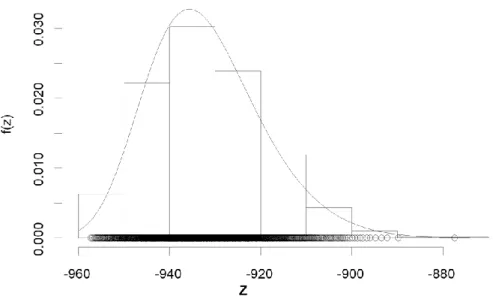
Figure 2.4 shows estimated generalized extreme distribution of log-likelihood, when sampling period n=50, and sampling time m=1000. The parameters for the distribution, μ, σ, and ξ, were estimated at -937.19, 11.33 and -0.13, respectively. Since, the log-likelihood of the tested graph is -862.39 resulting the GCP is 6.87e-7, the tested model is extremely significant in terms of GEV.

(19)

17

Figure 2.4 Estimated generalized extreme distribution of log-likelihood.

The values of likelihoods calculated based on the model in Figure 2.3 are denoted by each bin, and the estimated density function of the generalized extreme distribution is denoted by a curve.

Figure 2.5 Null distribution for log-likelihood in randomized graphs.

The values of the log-likelihoods calculated based on the model in Figure 2.3 are denoted by each bin.

Log-likelihood

Frequency

-960 -940 -920 -900 -880

0100020003000400050006000

(20)

18

Figure 2.5 shows that log-likelihood distribution when Nr=50000 with the nonparametric method. The log-likelihood of the tested graph is -862.39, and the GCP is less than 1.0e-5. In nonparametric method, the tested graph also shows statistically significance.

On the other hand, the likelihood of a false network shown in Figure 2.6 is -954.61, and the GCP is 9.8e-1. This result indicates that the GCP precisely reflects consistency according to the network structure.

Figure 2.6 A false network structure.

Thus, the nonparametric method also successfully worked. In the following analysis, we use the nonparametric method to estimate the GCP because of its simplicity.

In the following sections, we will demonstrate that proposed method does not depend on network topology, a number of data points, noise level, and noise distribution.

2.6 Robustness in Terms of the Dimensions of the Analyzed Data

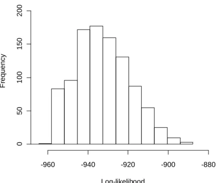
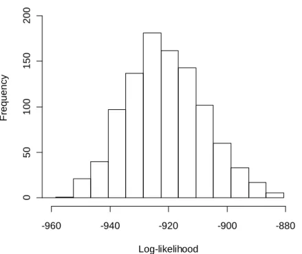
We test the robustness of our method in terms of the number of data samples for one variable (data dimension) that is smaller than the data dimension ({Xi} for i=1,2,...,50) in above simulation study (see section 2.5). This is because the experimental samples are frequently limited, especially in molecular biology, due to the technical difficulty of performing experiments or samplings. Thus, situations in small data dimensions are expected in the actual data. We performed the same estimation of GCP as that in Figure 2.3, by using the data with 15 and 30 dimensions, and in both cases, the present method operated well (Figure 2.7, Figure 2.8). On the estimated null distributions, the GCPs in the both cases were less than 1.0e-4.

(21)

19

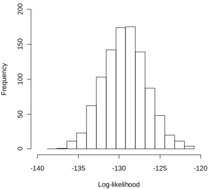
Figure 2.7 Distribution of log-likelihood using the data with 15 dimensions.

Figure 2.8 Distribution of log-likelihood using the data with 30 dimensions.

Log-likelihood

Frequency

-140 -135 -130 -125 -120

050100150200

Log-likelihood

Frequency

-290 -285 -280 -275 -270 -265 -260

050100150200

(22)

20

2.7 Robustness in Terms of the Magnitude of Noise in the Analyzed Data

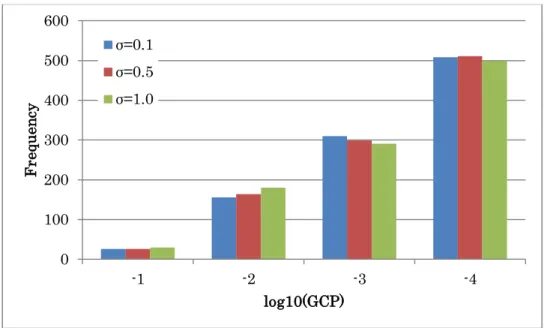
We estimated the GCP in various noise ranges. For this purpose, the value of the standard deviation in the structural equations for data generation: σ=0.1 (see section 2.5) was changed to two values: σ=0.5 and 1.0. The data dimension for this study was set to 15. We calculated 100 GCPs for the three ranges of standard deviations with same network in section2.5 (Figure 2.3) and the total number of randomly generated graphs Nr=1000. Finally, the probabilities of the generated graphs were calculated. The histograms of the GCPs in the three ranges of standard deviations are shown in Figure 2.9.

Figure 2.9 Histograms of the GCPs with different level of standard deviation.

The log-values of graph consistency probabilities calculated based on the model in Figure 2.3 are denoted by each bin for three levels of standard deviations.

In this figure, 1000 GCPs were plotted against the number of connections in the generated graphs that were different from those in the examined graph in the respective cases of standard deviations. The result shows that the GCPs were increased according to their noise level. The noise is amplified as the number of parents grows in the present simulation. For example, the standard deviation is (α12+α22+1)σ, when a descent has two parents and αi is the path coefficient between the descent and the i-th parent. About 97%

GCPs were less than 0.1 in this simulation study, which indicate that the present method enable us to detect true network with high frequency.

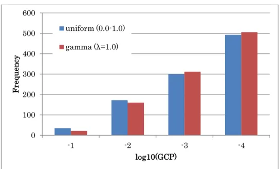
In addition, we assumed that the distribution of the data noise also follows uniform and gamma distribution like exponential (Figure 2.10), and obtained similar results in

0 100 200 300 400 500 600

-1 -2 -3 -4

Frequency

log10(GCP) σ=0.1

σ=0.5 σ=1.0

(23)

21

terms of the robustness about the data noise (Figure 2.11).

Figure 2.10 Distributions of uniform (0:1) and gamma (λ=1.0).

Probability density functions of uniform and gamma distributions are described.

Figure 2.11 Histograms of the GCPs with different distribution of data noise.

The log-values of graph consistency probabilities calculated based on the model in Figure 2.3 are denoted by each bin for uniform and gamma distributions.

Note that we also examined above studies with 100 data dimension, and then all the GPCs were less than 1.0e-4, which indicate that in case of relativity large observation, our method can perfectly detect the true network without depending on noise level and distribution. At any rate, careful preprocessing of the measured data may be required to apply our method to actual data depending on the number of observations.

0.0 0.2 0.4 0.6 0.8 1.0

0.60.81.01.21.4

x

f(x)

0 2 4 6 8 10

0.00.20.40.60.81.0

x

f(x)

0 100 200 300 400 500 600

-1 -2 -3 -4

Frequency

log10(GCP) uniform (0.0-1.0)

gamma (λ=1.0)

(24)

22

2.8 Robustness Regarding the Variation of the Network Structure

We further examined effect of network topology on the present method. We applied the present method to the three network structures shown in Figure 2.12, Figure 2.13 and Figure 2.14 with same condition of section2.5.

Figure 2.12 A tested network with chain structure like metabolic pathway.

Figure 2.13 A tested network with tree structure like gene regulatory network.

Figure 2.14 A tested network with cascade structure like signal transduction pathway.

The three networks are analogous to the typical structures of biological networks; the first Figure 2.12 is analogous to part of a chain reaction in a metabolic pathway, the second Figure 2.13 represents the simple structure of a gene regulatory network, and the

(25)

23

third Figure 2.14 depicts a cascade in a signal transduction pathway. According to the connectivity in the network, the data were generated with the corresponding structural equations, and the present method was applied to estimate the graph consistency with the generated data. All the GCPs were less than 1.0e-4, which indicate that the present method operated well in all of the network structures (Figure 2.15, Figure 2.16, Figure 2.17).

Here, the forms of distribution for three networks were slightly different. This may be caused by the structural diversity of randomized graphs depending on the original network topology. However, as mentioned previous section, the nonparametric method enables us to estimate precise GCP without consideration of the likelihood distribution form. This simulation shows that the present method can be applied to various structures of networks.

Figure 2.15 Distribution of log-likelihood using the chain network corresponding to Figure 2.12.

The values of log-likelihoods calculated based on the model in Figure 2.12 are denoted by each bin.

Log-likelihood

Frequency

-960 -940 -920 -900 -880

050100150200

(26)

24

Figure 2.16 Distribution of log-likelihood using the tree network corresponding to Figure 2.13.

Figure 2.17 Distribution of log-likelihood using the cascade network corresponding to Figure 2.14.

Log-likelihood

Frequency

-960 -940 -920 -900 -880

050100150200

Log-likelihood

Frequency

-950 -940 -930 -920 -910 -900

050100150200

(27)

25 2.9 Pitfalls of our method

Our approach has some pitfalls mainly due to network structual restriction. As defined in previous section (see section 2.1), our model is based on the DAG. However, there are many feedback and undirected relations in actual biological systems, our method cannot treat them. Therefore, the limitaiton may overlook important discoveries. In adition, our approach requires genereting a plenty of randomized networks to create background null distribution of likelihood for evaluating a query network. However, when a query topology is dense, especially in near full model, there is insufficinet space on unique random network structures to describe the background distribution.

Fortunately, becasue biological systems frequently form quite sparse network, which have charactors like small-world [47] and scale-free [48] properties, in many cases, we can obtain sufficent number of randomized networks.

2.10 Network Screening

In the previous sections, we show that the GCP reflects consistency of a pair of graph and measured data by the simulation study. However, we frequently encounter in cases where a tested graph structure cannot be determined or assumed. For example, in general, when a cell is stimulated by a particular signal, then it is not obvious that which network response to the signal in a vast amount of regulatory networks in cells.

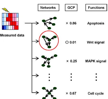
Therefore, a technique to detect active networks in pre-defined many functional networks is important. We define this concept named "Network screening" (Figure 2.18).

Fortunately, large informative databases for metabolic pathways, signal transduction networks and transcriptional networks are becoming increasingly available [39][40][41].

Thus, we can perform the network screening by combination of the GCP and those databases.

(28)

26

Figure 2.18 Schematic diagram of the network screening.

The graph consistency probabilities (“GCP”) between the network structures (“Networks”) characterized by biological functions (“Functions”) and the measured data (“Measured data”) are estimated. The network structure with a significant probability (GCP<0.05) is denoted by a red circle.

2.11 Demonstration of GCP and Network Screening with Actual Data

Here, we examined the performance of the present method with two sets of actual networks in Escherichia coli and the corresponding actual measured data. One set is a regulatory network for the SOS response system with the promoter activity of the constituent genes measured by green fluorescent protein (GFP) [49], and the other is 30 networks classified by gene functions, with the gene expression under anaerobic conditions measured by microarray [50]. The former examination is a verification of the GCP method for an actual network, and the latter is a demonstration of the network screening as a high-throughput search of network candidates, which consistent with the data measured under particular conditions.

2.11.1 Evaluation of Escherichia coli SOS Network

The gene network in the SOS DNA repair system is schematically shown in Figure 2.19.

It is a well-characterized transcriptional network in Escherichia coli [51][52].

(29)

27

Figure 2.19 SOS DNA repair transcriptional network.

The network structure is cited from[51][52]. See each gene function of the network in the text.

One of the SOS genes, RecA, acts as a sensor of DNA damage, and a master repressor (LexA) binds sites in the promoter regions of these operons. The corresponding data to the constituent genes in the network are measured with real-time monitoring by means of low-copy reporter plasmids, in which a promoter controls green fluorescent protein [49]. By using our method, the GCP of the SOS network with the corresponding measured data was estimated at 0.049, and the network structure was estimated to be consistent with the data measured from the examined network. However, the GCP is slightly large in comparison with the GCPs in the simulation studies in the previous section 2.5. This is partly because the cyclic relationship of RecA is neglected in the examined network. At any rate, the performance of the present method was verified by a well-known actual network, with a size similar to that in the simulation study, and with the corresponding data measured by an experimental study.

2.11.2 Network Screening for Escherichia coli Networks under Anaerobic Conditions

Subsequently, we applied the network screening to practical data. We first classified transcription factors (TFs) and its regulated genes compiled in EcoCyc [53], according

to the classification scheme of gene functions

(http://biocyc.org/ECOLI/class-tree?object=Genes). Using the functional gene sets of the TFs and its regulated genes, we next reconstructed the networks, so as to the network to be “connected graph” (i.e., it contains a path between arbitrary two nodes).

Thus, we obtained 130 regulatory networks that are characterized by biological functions. The nodes which expression profiles were not found in expression data were excluded from the 130 networks. Since the network screening algorithm requires a certain number of nodes in the examined graph due to variety of structures for

(30)

28

randomize graphs, we removed the small networks with less than 8 edges, as a result, 30 networks were used for evaluation. The consistency of each of the 30 networks was estimated with expression profiles measured under 22 different anaerobic conditions (GSE1107) [50] cited from NCBI GEO [1]. The expression profiles were standardized by the average and the standard deviation in each condition (i.e. z-score normalization), as pre-processing of the measured data [54].

j j ij ij

Z x





  (15)

Where Zij and xij are the standardized and intact expression values of the i-th gene and the j-th sample, respectively, and μj and σj are the average and the standard deviation of all genes over the j-th sample, respectively.

Table 2.1 shows the network screening results with Nr=1000; the analyzed networks and the corresponding GCPs and estimated FDR (False Discovery Rate) q-values of the 30 networks. Here, we set significance level to GCP<0.05 and FDR q-value<0.25 (bold lines).

(31)

29

Table 2.1 Network screening result for E.coli under anaerobic environment.

The column “ID” shows the functional classification defined in EcoCyc database. The bold lines are significant networks (GCP<0.05 and FDR q-value<0.25).

The result shows that a variety of size of networks, “Carbon compounds”, “SOS response”, “DNA repair”, “Anaerobic respiration” and “Cytoplasm”, were significantly identified. Most significant network for “Carbon compounds” was identical to maltose regulon [55] (Figure 2.20).

ID Description Node Edge GCP FDR q-value

C9449 Carbon compounds 10 9 3.00E-03 8.00E-02

C9337 SOS response 11 10 7.00E-03 8.00E-02

C9354 DNA repair 11 10 8.00E-03 8.00E-02

C9490 Anaerobic respiration 89 161 1.10E-02 8.30E-02

C9376 Cytoplasm 12 11 2.70E-02 1.60E-01

C9340 Flagella 9 8 5.50E-02 2.80E-01

C9474 Nucleotide and nucleotide conversion 11 15 6.70E-02 2.90E-01

C9372 Transcription related 91 143 1.50E-01 5.40E-01

C9449 Carbon compounds 10 11 1.60E-01 5.40E-01

C9362 Nucleoproteins, basic proteins 9 8 1.90E-01 5.60E-01 C9331 Motility, chemotaxis, energytaxis 9 8 2.70E-01 7.30E-01

C9333 Detoxification 6 8 3.00E-01 7.50E-01

C9523 Activator 58 92 5.30E-01 1.00E+00

C9449 Carbon compounds 8 7 5.90E-01 1.00E+00

C9528 Repressor 52 77 6.30E-01 1.00E+00

C9426 Colanic acid (M antigen) 6 9 6.40E-01 1.00E+00

C9448 Amino acids 6 9 6.60E-01 1.00E+00

C9449 Carbon compounds 9 8 6.90E-01 1.00E+00

C9462 Amino acids, formyl-THF biosynthesis 7 10 6.90E-01 1.00E+00 C9448 Amino acids, formyl-THF biosynthesis 7 10 7.00E-01 1.00E+00

C9401 Tryptophan 9 8 7.80E-01 1.00E+00

C9376 Cytoplasm 10 9 8.20E-01 1.00E+00

C9509 Operon 6 9 8.70E-01 1.00E+00

C9383 Arginine 11 10 1.00E+00 1.00E+00

C9393 Isoleucine/Valine 13 12 1.00E+00 1.00E+00

C9394 Leucine 14 17 1.00E+00 1.00E+00

C9420 Purine biosynthesis 13 12 1.00E+00 1.00E+00

C9449 Crabon compounds 6 9 1.00E+00 1.00E+00

C9493 Fermentation 11 10 1.00E+00 1.00E+00

C9504 Phosphorous metabolism 23 22 1.00E+00 1.00E+00

(32)

30

Figure 2.20 Significant network: “Carbon compounds”.

The network structure for “carbon compounds” is described. See function of the network in the text.

Actually, this is unexpected result, because glucose utilization as carbon source for respiration is speculated from culture condition. This suggests a possibility of pH response, indicating activation of the maltose regulon depending pH in culture medium [56].

Every three significant network, “SOS response”, “DNA repair” and “Cytoplasm”, are based on lexA regulon, thus, several target genes are overlapped (blue nodes, recA, umuC-D, uvrA-D in Figure 2.21). Where, light blue, pink and green nodes are corresponding to “SOS response”, “DNA repair” and “Cytoplasm”, respectively.

Figure 2.21 Merged network of “SOS response”, “DNA repair” and “Cytoplasm”. The nodes with blue, light blue, pink and green are corresponding to “Common”, “SOS response”, “DNA repair” and “Cytoplasm” network, respectively.

The merged network structure for “SOS response”, “DNA repair” and “cytoplasm” is described. See function of the network in the text.

(33)

31

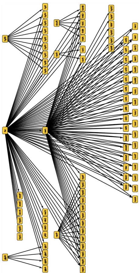
Indeed, the SOS response network is previously reported that it is activated under anaerobic condition [57], these lexA networks have possibility of playing some role in respiration in anaerobic circumstance. In Figure 2.22, “anaerobic respiration”, as the name suggests, is related for respiration under anaerobic condition, even though the network consists of a lot of genes, our method precisely detected its response. The gene encoding the transcription factor in the network is fnr, one of the seven global regulators in E. coli [58], and the modular controlled by its product, Fnr, encodes proteins involved in cellular adaptation to growth in anoxic environments [59][60][61]. Since the network is related to adaptations to environmental changes, many genes are comprehensively associated with each other, and the network structure is complex. These results show that the network screening is applicable for practical analysis with high confidence.

(34)

32

Figure 2.22 Significant network: “Anaerobic respiration”.

The network structure for “anaerobic respiration” is described. See function of the network in the text.