魚類の遡上行動を支配するHamilton-Jacobi-Bellman方程式の数理および数値解析 (非線形波動現象のメカニズムと数理)

Mathematicaland Numerical Analyses

on

a

Hamilton-Jacobi-Bellman Equation Governing Ascending Behaviour of Fishes

(邦題 :魚類の遡上行動を支配するHamilton-Jacobi-Bellman 方程式の数理および数値解析)

HidekazuYoshioka1,Koichi

Unami2,

and Masayuki

Fujihara2

1

Faculty of Life and Environmental Science, Shimane University Nishikawatsu-cho 1060, MatsueCity, ShimanePrefecture,690-8504,Japan

$E$-mail: voshih_{$(\partial 1ife.shimane-u.ac.i_{-}D-$}

2

Graduate School of Agriculture, Kyoto University

Kitashirakawa-Oiwake-cho, Sakyo-ku, KyotoCity,KyotoPrefecture,606-8502, Japan

$E$-mail:unami$(\partial adm.$_{$kvot\circ-u.ac.i_{-}D-$}kais. (K. Unami),fuiihara\copyright kais.kvoto-u.ac.$i_{-}D$(M.Fujihara)

Abstract

Ascending behaviour of individual fishes in 1-D open channels is considered

as

a

transport phenomenongovemed by

a

continuoustime stochasticprocessmodel. Astochastic control problemis formulated that determines the drift of the model based

on a

minimizationprinciple of physiological energy consumption of the fish during migration. The problem ultimately reduces to solving

a

Hamilton-Jacobi-Bellmanequation goveming the optimal ascending velocity, whichis

a

nonlinear and nonconservative parabolic partial differential equation. Mathematical and numerical analyses

on

the equation

are

performed for comprehending behaviour of its solutions. Some numerical issues encountered insolving theequation

are

alsodiscussed.

Key words: Ascendingbehaviour, stochastic differentialequation, stochastic control problem, energy

minimizationprinciple, Hamilton-Jacobi-Bellman equation, ascending condition 1. introduction

Ascending behaviour of fishes in

open

channels, such

as

rivers, agricultural drainage canals, and fishways, is a complicated transport phenomenon. Assessment ofascending behaviour of individual fishes is

one

of the most crucial hydro-environmental research topics because ofthe urgent need to

establish

an

effective framework for improving and preserving aquatic ecological systems where fishes play central roles. One example is designing

a

fishway passaging upstream and downstream

water bodies of

a

physical barrier, such

as

dams and headworks (Katopodis and Williams, 2012).

Another example is assessmentof ecological functions of surface water systemsserving

as

passages

and habitals forfishes, such

as

stream networks (Cote et al.,2009) and surface agricultural drainage

systems(Unamiet al.,2010).

Ascendingbehaviour of fishes is subject to inherent disturbances dueto

our

limited knowledge

and environmental and ecological stochasticity. Mathematical models

serve

as

effective

means

for

simulatinghydraulicprocesses in surfacewater bodies,which provide basic hydraulic information for

considering migration of fishes. Although a large number of researches discussed the hydraulic

processes, far less number of researches focused on migration offishes, _{mainly due}to difficultiesto findtheir reasonablemathematical expressions (Liao, 2007; Willis, 2011). It has been suggested that stochastic process models

are

effective for comprehending migration of fishes, in which the

stochasticity embedded in the dynamics is considered(FujiharaandAkimoto, 2010).Although these models are effective forassessingthe ascendingbehaviour offishes, they

assume

that the hydraulic

processes determine the behaviour without considering biological and ecological feedbacks, such

as

the physiological energy consumption of fishes during the migration (Brodersen etal., 2008). One possible way to develop

a more

reasonable model for ascending behaviour of fishes considering

hydraulics, biology, and ecology in a feedback

manner

is to formulate theproblem in the context of

optimalcontrolbased

on

the stochastic differential equation(SDE) ($\emptyset$ksendal, 2007);

however,such

a

Thepurpose ofthis paper is to presenta stochasticprocess model for ascending behaviour of

fishes,inwhichthehydraulic,ecological, biologicaleffects involvedinthedynamics

are

considered in

a

feedback

manner

based

on a

stochastic control theory. Lagrangian movement of individual fish is considered

as

a

controlled Markov process subject to shallow water flows. A stochastic control

problem is then formulated for determining the optimal ascending strategy that harmonizes the two

conflictingobjectives: minimization ofthetotal physiological energyconsumption and maximization

ofthe profit gained when reaching the upstreamarea.

2. Stochasticprocessmodel

This

paper

focuses exclusively

on

1-Dproblems. The domain ofwaterflows isthe 1-Dopenchannel

$\Omega=(0,L)$ with its lengh $L(>0)$ and water depth $h(>0)$

.

The flow velocity of water in the

channelis denotedby $V$,whichis assumedto beunidirectionaland its positivedirectionis

same

with

that ofthe $x$ abscissadefined along the channel $(V>0)$

.

The upstream- and downstream- ends of

the channel

are

$x=0$ _and $x=L$, respectively. The position of individual fish at the time $t$ is

denoted by $X_{t}$, whichis

a

continuous time stochastic process. Inspiring from the stochastic process

modelforLagrangianmovementof solute particles (Yoshiokaand Unami, 2013),the SDE goveming

$X_{l}$ is proposed

as

$M_{t}=(V-u)dJ+\sqrt{2D}dB$_{, (1)}

where $B$, isthe 1-D standard Brownianmotion ($\emptyset$ksendal, 2007), $u$ isthe ascending speed offish

where its positive direction is taken

same

with that of $-x$, and $D(>0)$ is the dispersivity that

modulates the magnitude of the stochasticity involved in the dynamics, which should be related with turbulent intensity of the flow. The ascending velocity $u$ isthecontrol variable of themodel, which is assumedtobeconstrained in the admissibleset

$U=\{u\Vert u|\leq u_{M}\}$ (2)

forapositive constant $u_{M}$ that

can

be naivelytaken

as

themaximum swimming speed offishes, but

wouldactually varyin both space and timedepending

on

hydraulic andbiological conditions. In this

paper, $u_{M}$ is assumed to be constant for the sake ofbrevity and is referred to

as

the maximum swimming speed. The coefficients $V$ and $D$

are

assumed not to involve the control variable $u.$

The generator $A$ ofthecoupled stochastic process $Y_{l}=(t,X_{t})$ conditioned on $Y_{s}=(s,x)$ is given

by($\emptyset$ksendal,2007)

$AY= \frac{\partial y}{\partial s}+(V-u)\frac{\partial y}{\ }+D \frac{\partial^{2}y}{\partial x^{2}}$ (3)

for

a

sufficiently regular function $y=y(s,x)$

.

3. Stochastic controlproblem

3.1 Hamilton-Jacobi-Bellmanequation

Astochastic control problemis formulated in ordertodeterminethe ascending velocity $u$

.

Literatures

indicate that fishesminimize physiological energyconsumptionduring migrationdependingon local

hydraulic conditions (Brodersen et al., 2008). Assuming that the fish strategically ascends the open

channel $\Omega$ toward the upstream boundary $x=0$ based on a physiological energy consumption

minimizationprinciple, inwhichthevaluefunction $J^{u}$ to bemaximized isproposed

as

$J^{u}(s,x)= E^{S,X}[\int_{S}^{\overline{T}}(-\frac{1}{2}u^{2})dt+G(\overline{T},Y_{\overline{T}})]$ with $\overline{T}=\min(T,\tau^{s.x})$ (4)

where $E^{s,x}[\cdot]$ representstheexpectation conditionedon $Y_{s}=(s,x)$, $T$ is the terminaltime, $\tau^{s,x}$ is

the first exit time of the process $Y_{t}$ from the spatio-temporal domain $–=\Omega\cross(-\infty,T)$, and $G(\geq 0)$

3.2 Ascending condition

The ascending condition of the fish is defined

so

that

passage

efficiency ofthe channel $\Omega$

can

be

analyticallyassessed with thepresentmodel. The ascending condition in this

paper

is givenby

$V_{g}=V-u<0$ in $\Omega$, (14)

which

means

that the ground velocity $V_{g}$ ofthe fish with the optimal ascending velocity $u$ is

negative (is directed toward the upstream) everywhere in the channel $\Omega.$

$Eq.(14)$ is rewritten with

Eq.(9)

as

AccordingtoEq.(14), fishes do not ascend the channel if $V-u_{M}>0$ in $\Omega$

.

Such

a

trivial condition

isoutoftheinterestofthispaperand thecondition $V-u_{M}\leq 0$ is assumedtobesatisfiedin $\Omega.$

4. Mathematical analysisontheHJBE

Mathematical analysis

on

the HJBE(13) isperformed. The HJBE(13) is non-dimensionalizedforthe sake ofbrevity ofthe analysis.Eqs.(12) and (13)

are

non-dimensionalized

as

$(1+w) \frac{d\phi}{dy}+\frac{1}{p}\frac{d^{2}\phi}{dy^{2}}-\frac{1-\chi}{2}w_{M}^{2}=0$ (16)

and

$w= \frac{\chi}{2}\frac{d\emptyset}{dy}+(1-\chi)w_{M}sgn(\frac{d\emptyset}{dy})$, (17) respectively,using the non-dimensional variables

$y= \frac{x}{L},$ $\emptyset=\frac{\Phi}{VL},$ $w_{M}= \frac{u_{M}}{V},$ $p= \frac{VL}{D}$,and $P_{0}= \frac{P}{VL}$

.

(18)

Thefollowing two

cases

$w_{M}$

are

considered in thispaper,which

are

Case(a): $w_{M}=+\infty$ ($u_{M}=\dashv\infty$:unboundedcase)

and

Case(b): $0<w_{M}<+\infty$ ($0<u_{M}<+\infty$:boundedcase).

4.1 Case(a):unbounded

case

$(w_{M}=+\infty)$

This is

an

idealized

case

where the admissible set $U$is identified with the 1-D space. $\mathbb{R}$ although it

has been indicated that there certainly exists

an

upper bound of the maximum swimming speed for

each fish(IosilveskiiandWeihs,2008). Inthis case,Eqs.(16) and (17) reduce to

$(1+ \frac{1}{2}\frac{d\emptyset}{dy})\frac{d\emptyset}{dy}+\frac{1}{p}\frac{d^{2}\emptyset}{dy^{2}}=0$

.

(19)

Assuming thatEq.(19) has

a

classicalsolution,applicationofthevariabletransformation

$\psi=e$

理

(20)

toitleads to

$\frac{d\psi}{dy}+\frac{1}{p}\frac{d^{2}\psi}{dy^{2}}=0$, (21)

whichisanalytically solvable. The modelis therefore tractable inthis

case.

If $P_{0}\neq 2$,the solutionto

Eq.(21) isanalyticallyderivedwiththe transformedboundaryconditions

$\psi(0)=e^{\frac{pP_{0}}{2}}$

and $\psi(1)=1$ (22)

as

$\psi=\frac{1-e^{p(\frac{P_{0}}{2}1)}+(e^{\frac{pP_{0}}{2}}-1)e^{-py}}{1-e^{-p}}$

.

(23)

ByEqs.(20) and $(23\rangle, the$solution$to Eq.(19)$ is derived

as

withitsgradient

$\frac{d\emptyset}{dy}=\frac{2(e^{\frac{pP_{0}}{2}}-1)}{(e^{F(\frac{P_{0}}{2}1)}-1)e^{\mathscr{O}}-(e^{\frac{pP_{0}}{2}}-1)}$

.

(25)

The steady solution for $P_{0}=2$ is derived with the application of the L’Hospital’s rule to Eq.(24),

whichisgiven by

$\emptyset=2-2y$ (26)

withitsgradient

$\frac{d\phi}{dy}=-2$

.

(27)

For $p>>1$ and $P_{0}>2$,themaximumabsolutevalueofthegradient $\frac{d\emptyset}{dy}$ isevaluated

as

$| \frac{d\emptyset}{dy}|_{y=I}=-\frac{d\emptyset}{dy}|_{y=I}=o(e^{P(\frac{P_{0}}{2}1)})$, (28)

indicatingthat thereexists

a

boundary layer

near

$y=1$ with thewidth of $o(e^{-p(\frac{P_{0}}{2}I)})$

.

Figures $1(a)$

and $1(b)$ show profiles ofthe solution (25) for different values of $p$, showing thatthere certainly

exists

one

sharp boundary layer in each solution profile. According to Eq.(14), the optimal ground

velocity $V_{g}$ inthepresent

case

diverges

near

$y=1$

as

$p$ increases.

o.o

0.5 1.0

o.o

0.5 $\iota.\mathfrak{o}$

$Di\infty Ioe$ $Di\Phi ICG$

Figure 1: Steady solutionsinEq.(24) with(a) $p=10$ and(b) $p=100$ fortheboundaryvalues $P_{0}=0.1$ and

$P_{0}=1,2\ldots,10$.The solutionsarenormalizedwith $P_{0}.$

ByEq.(25),thesolution (24) satisfiesthe ascending condition

$1-w. =1+ \frac{d\emptyset}{dy}<0$ (29)

if

$P_{0}> \frac{2}{p}\ln(\frac{1+e^{p}}{2})$

.

(30)

Eq.(30) issatisfied if

$P_{0}\geq 2$, (31)

which does not depend

on

the parameter $p$

.

The right-hand side of Eq.(30) is a non-increasing

(or equivalently

as

$D$ increases), indicating that the increase of turbulence would enhance the

ascending behaviour of fishes.Eq.(31) isrewritten in

a

non-dimensional form

as

$P\geq 27\mathcal{I}$, (32) showing that the fishes ascend the channel $\Omega$ iftheprofit gained when reaching the upstream-end

$y=0$ issufficiently large forfixed $V$ and $L.$

4.2 Case(b):bounded

case

$(w_{M}=+\infty)$

Inthiscase,Eqs.(12) and (13) reduceto

$(1+ \frac{1}{2}\frac{d\emptyset}{dy}I\frac{d\emptyset}{dy}+\frac{1}{p}\frac{d^{2}\emptyset}{dy^{2}}=0$ (33)

if $\chi=1$ andto

$\frac{d\phi}{dy}+w_{M}|\frac{d\phi}{dy}|+\frac{1}{p}\frac{d^{2}\phi}{dy^{2}}-\frac{1}{2}w_{M}^{2}=0$ (34)

if $\chi=0$

.

Straightforward calculations show that the condition $\chi=1$ issatisfied

over

$\Omega$ if

$P_{0}\leq 2\leq w_{M}$

.

(35)

Similarly, the condition $\chi=0$ is satisfied

over

thedomain $\Omega$ if

$1<w_{M}<2$ and $2< \frac{w_{M}^{2}}{2(w_{M}-1)}<P_{0}$

.

(36)

Application of

an

elliptic maximum principle to Eq.(34) leads to $\frac{d\emptyset}{dy}<0$ in

$\Omega$,

which reduces

Eq.(34) to

$(1-w_{M}) \frac{d\phi}{dy}+\frac{1}{p}\frac{d^{2}\phi}{dy^{2}}=\frac{1}{2}w_{M}^{2}$. (37)

Bq.(37) has the analyticalsolution

$\emptyset=P_{0}+\frac{w_{M}^{2}}{2(w_{M}-1)}y-(P_{0}+\frac{w_{M}^{2}}{2(w_{M}-1)})\frac{e^{p(w_{M}-1)y}-1}{e^{p(w_{M}-1)}-1}$ (38)

withitsgradient

$\frac{d\emptyset}{dy}=\frac{w_{M}^{2}}{2(w_{M}-1)}-p((w_{M}-1)P_{0}+\frac{w_{M}^{2}}{2})\frac{e^{p(w_{M}-1)y}}{e^{p(w_{M}-1)}-1}<0$, (39) showing that the solution (38) satisfies the ascending condition if $w_{M}>1$, namely ifthe maximum

swimmingspeed $u_{M}>1$ islarger than the flow velocity $V$

.

Althoughnot presented in thispaper, it

has been numericallyconfirmedthatthesolution $\phi$ satisfies the ascending condition if both _{$P_{0}>2$}

and $w_{M}>2$

are

satisfied. Maximum absolutevalueofthegradient $\frac{d\emptyset}{dy}$ is evaluated

as

$| \frac{d\emptyset}{dy}|_{y=1}=-\frac{d\emptyset}{dy}|_{y=1}=O(p)(p>>1)$, (40)

indicating that there exists a boundary layer near $y=1$ for sufficiently large $p$, but which is less

sharp compared withthatin the unbounded

case

where thelayerhas exponential width. Figures 2(a)

and 2(b) show the solutionsto the HJBE in the bounded

case

with $w_{M}=1.5$ for different values

of.

$p$. Similarly, Figures 3(a) and 3(b) showthe solutions with $w_{M}=2.5$. Figures 2 and 3 show that

thereexists

one

sharpboundary layerin each solutionprofilebut isnotapparentlysharper than that in

thecorresponding unbounded

case

subject tothe

same

values of $p$ and $P_{0}$ inFigure 1. Figures 2

o.o

$\mathfrak{o}.5$ 1.0 $0.\mathfrak{o}$ 0.5 1.0

$Dis\infty nc\epsilon Dis\alpha nc.$

Figure2:Steady solutions in the boundedcasefor $w_{M}=1.5$ with(a) $p=10$ and(b) $p=100$ for the

boundary values $P_{\mathfrak{o}}=0.1$ and _{$P_{0}=1,2\ldots,10$}

.

The solutionsarenormalized with $P_{0}.$

o.o

0.5 1.0 $\mathfrak{o}.\mathfrak{o}$

0.5 1.0

$Dis\alpha nc.

DiS\mathfrak{g}nCe$

Figure3:Steadysolutionsintheboundedcasefor $w_{M}=2.5$ with(a) $p=10$ and(b) $p=100$ for the

boundary values $P_{0}=0.1$ and $P_{0}=1,2\ldots,10$.The solutionsarenormalized with $P_{\mathfrak{o}}.$

If the twoparameters $P_{0}$ and $w_{M}$ satisfy neitherEqs.(35)

nor

(36),then theremayexistatleast

one

point $\sigma\in\Omega$ serving

as

the interface of the sub-domain with $\chi=0$ and that with $\chi=1.$

Numerical simulations for

a

variety of theparametervalues $(P_{0},p)$ suggest thatthereexistsat most

one

$\sigma$ for each solution profile with fixed $(P_{0},p)$

.

It has also been numerically checked that the

solution is such that $\chi=1$ in $(0,\sigma)$ and $\chi=0$ in $(\sigma,1)$ if _{$w_{M}>2$}, and $\chi=0$ in $(o,\sigma)$ and

$\chi=1$ in $(\sigma,1)$ if _{$w_{M}<2$}

.

Noanalyticalexpression of $\sigma$ has been derived

so

far.

Underthe other conditions in the bounded case, analytical solution to the HJBE isnotavailable.

In addition, regularity of the solution to the HJBE in such

cases

is not

a

trivial issue and

comprehending its mathematical properties requires the

use

of

an

appropriate mathematics. In this paper,aregularization method for the HJBEispresented for smoothnessofits solution,whichis later

implementedintoanumerical method. Firstly, the function $h_{K}=h_{K}(a)$ is defined

as

$h_{K}=\{\begin{array}{l}a(|a|\leq K)Ksy1(a)(|a|>K)\end{array}$ (41)

withitsgradient

$\frac{\partial h_{K}}{\partial a}=\{_{0}^{1}(|a|>K)(|a|\leq K)$ (42)

where $K(>0)$ _is

a

_{positive, bounded constant.} Eqs.(41) and (42) show that $h_{K}$ and $\frac{\partial h_{K}}{\partial a}$

are

$\chi_{\epsilon}=H_{\epsilon}(\frac{d\emptyset}{dy}+w_{M})-H_{\epsilon}(\frac{d\phi}{dy}-w_{M})$, ₍₄₃₎ where $\epsilon$ is a sufficiently small positive constant and

$H_{\epsilon}$ represents the regularized Heaviside

function

$H_{\epsilon}(a)= \frac{1}{2}(1+\tanh(\frac{a}{\epsilon}))$ ₍₄₄₎

whosepartial derivative $\frac{\partial H_{\epsilon}}{\partial a}$ isbounded

as

$(0<) \frac{\partial H_{\epsilon}}{\partial a}=\frac{1}{\epsilon\cosh^{2}(\frac{a}{\epsilon})}$

.

(45)

ByEq.(45),theconditions

$|a \chi_{\epsilon}|,|a\frac{\partial\chi_{\epsilon}}{\partial a}|<+\infty$ (46)

are

derived.Thirdly,definethefunction $f$ as

$f=(1+w_{\epsilon})a- \frac{1-\chi_{\epsilon}}{2}w_{M}^{2}$ ₍₄₇₎

with theregularized $w$ givenby

$w_{\epsilon}= \frac{1}{2}\chi_{s}h_{K}-(1-\chi_{\epsilon})w_{M}$, ₍₄₈₎ whichisbounded because

$|w_{\epsilon}|=| \frac{1}{2}\chi_{\epsilon}h_{K}-(1-\chi_{\epsilon})w_{M}|\leq\frac{1}{2}|h_{K}|+w_{M}<$十力．(49)

Thepartialderivative $\frac{\partial w_{\epsilon}}{\partial a}$ isexpressedas

$\frac{\partial w_{\epsilon}}{\partial a}=\frac{\partial}{\partial a}(\frac{1}{2}\chi_{\epsilon}h_{K}-(1-\chi_{\epsilon})w_{M})=\frac{1}{2}(\frac{\partial\chi_{\epsilon}}{\partial a}h_{K}+\chi_{\epsilon}\frac{\partial h_{K}}{\partial a})+\frac{\partial\chi_{\epsilon}}{\partial a}w_{M}$, (50)

which leadsto

$|a \frac{\partial w_{\epsilon}}{\partial a}|=|\frac{1}{2}(a\frac{\partial\chi_{s}}{\partial a}h_{K}+\chi_{\epsilon}a\frac{\partial h_{K}}{\partial a})+a\frac{\partial\chi_{\epsilon}}{\partial a}w_{M}|\leq\frac{1}{2}|a\frac{\partial\chi_{\epsilon}}{\partial a}||h_{K}|+\frac{1}{2}|a\chi_{\epsilon}||\frac{\partial h_{K}}{\partial a}|+w_{M}|a\frac{\partial\chi_{\epsilon}}{\partial a}|<+\infty$. (51)

Eqs.(49), (50),and (51) lead to.

$| \frac{\partial f}{\partial a}|=|1+w_{\epsilon}+a\frac{\partial w_{\epsilon}}{\partial a}+\frac{1}{2}w_{M}^{2}\frac{\partial\chi_{\epsilon}}{\partial a}|<1+w_{\epsilon}|a\frac{\partial w_{\epsilon}}{\partial a}|+\frac{1}{2}w_{M}^{2}|\frac{\partial\chi_{\epsilon}}{\partial a}|<+\infty$

.

(52)

ByEq.(52) and the Schauder’s fixedpointtheorem,theregularizedHJBE,which isgivenby

$(1+w_{\epsilon}) \frac{d\emptyset}{dy}+\frac{1}{p}\frac{d^{2}\emptyset}{dy^{2}}-\frac{1-\chi_{\epsilon}}{2}w_{M}^{2}=0$ (53)

witha non-zero $\epsilon$ has auniqueclassical solution subject tothe boundary conditions because

it has

the bounded driftand

source

terms inthe

sense

ofYamomotoandOishi(2006).Anumericalanalogue

ofthepresentregularizationis used in thefollowingsection.

5. Numericalanalysis

on

theHJBE

This section focuses

on

numerical simulation ofa HJBE in a periodic open channel, which

can

be

regarded

as

afishway having alongitudinally periodicstructure. Numerical issues encounteredwhen

solving the HJBE

are

also discussed. The channel $\Omega$ is assumed to be infinitely long and have

a

et al. 2015, in press). According to the computational results from a priori performed numerical

simulations, it has been indicated that

a

numerical counterpart of the regularizationmethodpresented

in Section 4.2 is crucial for solvingtheHJBE(60). Ifthe CPGFEM without theregularizationmethod

is usedfor solving Eq.(60), its numerical solutions involve spurious oscillations and/or_unphysically

flattenprofiles. Ithas been confirmed that the choice $K=0.2(\Delta y)^{-1}$ _where $\Delta y$ representsthe mesh

size_{gives reasonable numerical solutions for sufficiently fine meshes}$(\Delta y<0.0025)$

.

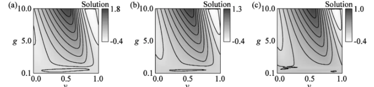
Figures 4(a) _through 4(c) _{show the numerical solutions in the 2-D phase space $(y,g)$ with}

$p=5$ for different values of_{the non-dimensionalized maximum swimming speed}

$w_{M}$

.

Similarly,

Figures 5(a) through 5(c) show the computed optimal ground velocity $V_{g}$ in the 2-D phase space

$(y,g)$ _with $p=5$ _{for different values of} $w_{M}$

.

The computational results show that the ascending

condition_{is satisfied for sufficiently high valuesof the trend} $g$

.

The computational

cases

withlower

and higher values of $p$ have also beenperformed. The results withthelower values of _$p(p=0.5$

and $p=1)$

are

_{qualitatively}

same

_{with those in Figures 4 and 5 except for that the numerical} solutions are much smoother. On the other hand, the numerical solutions forthe high values of $p$

$(p\geq 10)$exhibitlongitudinal_{oscillations,whichareconsideredtobe numericalartifacts.}

$y$ $y$ $y$

Figure4:Steadysolutionsinthe boundedcasefor $p=5$ and thetrend $0.1\leq g\leq 10$ with_(a) $w_{M}=5$, (b)

$w_{M}=6$,and(b) $w_{M}=7$.Thecounterscorrespondtotheten-section_{lines ofthemaximumandminimum}

values.

ア $y$ _ア

Figure5: The optimalgroundspeedintheboundedcasefor $p=2$ andthetrend O.$1\leq g\leq 10$

with(a) $w_{M}=5$,(b) $w_{M}=6$,and(b) $w_{M}=7$

.

The black linescorrespondto the contour line for _{$V_{g}=0.$}

6. Conclusions

Astochastic process model for analytical assessment of ascendingbehaviourofindividual fishes

was

proposedand basicproperties ofits solutions

are

investigatedbothfrom analytical and numerical point

ofviews.A regularized counterpart has also beenpresented and

was

applied to numerical simulation

of ascending behaviour of fishes in

a

longitudinally periodic channel. Although the presented

analytical solutions

are

for the dynamics underthe simplified cases, theywould

serve

as basics for comprehending mathematical properties ofthe HJBE.

Inthis paper, the model

was

applied to the problems in 1-D open channels. Extension ofthe

hydraulic properties

are

appropriately distributed, is possible if intemal boundary conditions

are

appropriately specified at junctions. Horizontally 2-D counterpart of the model has already been

proposed in Yoshioka et al. (2014b) where the flow field is computed with the 2-D shallow water

equations. Otherproblemsnotfocused

on

in thispaperinvolve migrationoffishschools,which

can

be

at least partially solved with

an

altemative SDE based

on

an

appropriate

mean

field approximation technique. Migration with moving and resting regimes, which isatypical behaviouroffishes,

was

not

addressed

as

well. This research topic will be addressed with

a

regime-switching diffusion process model that the authors recently developed, which is

a

continuous time SDE coupled with

a

discrete-state Markov

process

$(Yin and Zhu, 2010;$_Yoshioka$et al., 2014a)$

.

Acknowledgements:Thisresearch is supportedby JSPSundergrant No. $25\cdot 2731$

.

The authorsthank

to Dr. KenMori for his valuable suggestions andcomments

on

this research.

References

[1] Brodersen, J., Nilsson, P.A., Ammitzbll, J., Hansson, L.A., Skov, C., and $Br6$nmark, C.₍₂₀₀₈₎

Optimal swimming speed in head currentsand effects

on

distancemovementofwinter-migrating

fish,PLOSONE,Vol.3, No.5,$7pp$

.

DOI: $10.1371\Gamma_{j}ouma1.$pone.$0002156.$

[2] Cote, D., Kehler, D.G., Boume, C., and Wiersma, YF. (2009) A

new

measure

of longitudinal

connectivity forstreamnetworks,LandscapeEcology, Vol.24,No. 1,pp. 101-113.

[3] Fujihara, M. and Akimoto, M. (2010) A numerical model of fish movement in

a

vertical slot

fishway,Fisheries Engineering,Vol.47,No. 1,

pp.

13-18.

[4] Iosilveskii, G. andWeihs, D. (2008) Speed limits

on

swimming of fishes and cetaceans,Journal

ofthe

RoyalSociety, Interface, Vol.5, No. 20,pp. 329-338.

[5] Katopodis, C.andWilliams,J.G.(2012)Thedevelopmentsof fishpassageresearch in

a

historical

context,Ecological Engineering, Vol. 48,pp. 8-18.

[6] Liao, J.C. (2007) A review of fish swimming mechanics and behaviour in altered flows,

Philosophical Transactions

_ofthe

RoyalSociety(BiologicalSciences),Vol.362,pp. 1973-1993.

[7] $\emptyset$ksendal,B.(2007)Stochastic

Differential

Equations,Springer-Verlag,Berlin, 1-167.

[8] Unami, K., Ishida, K., Kawachi, T., Maeda, S., and Takeuchi, J. (2010) A stochastic model for

behavior offishascending

an

agriculturaldrainage system,Paddyand WaterEnvironment, Vol.8, No.2,pp. 105-111.

[9] Willis, J. (2011) Modelling swimming aquatic animals in hydrodynamic models, Ecological

Engineering, Vol. 222,pp. 3869-3887.

[10]Yamamoto, T. and Oishi, S. (2006)Amathematical theory for numerical treatment of nonlinear

two-pointboundaryvalue problems, Japan Joumal of IndustrialandAppliedMathematics,Vol. 23,

No. 1,pp. 31-62.

[11]Yin, G.G. and Zhu, C. (2010) HybridSwitching Diffiions, Springer Science$+$Business Media,

LLC,pp. 1-67.

[12]Yoshioka, H. and Unami, K. (2013) A cell-vertex finite volume scheme for solute transport

equations inopenchannelnetworks,ProbabilisticEngineeringMechanics,Vol.31,pp. 30-38.

[13]Yoshioka, H., Unami, K.,andFujihara, M.(2014a)A regime-switchingdiffusionprocessmodel

for longitudinal dispersion phenomena in vegetated open channels, Proceedings

_of

the $63rd$

NationalCongresson Theoretical andAppliedMechanics,OS-15-02-03,pp. 1-2.

[14]Yoshioka, H., Unami, K., and Fujihara, M. (2014b) A stochastic process model for ascending

behaviour of fishes infishways, Proceedings

_of

the $22nd$_{JapanRainwater Catchment Systems}

Association Congress,pp.31-36.

[15]Yoshioka, H., Unami, K.,and Fujihara, M.(2015) Mathematical analysis

on

a

conformingfinite

element scheme for advection-dispersion-decay equations

on

connected graphs, Journal ofJapan Society

_of

Civil Engineers(Specialissue

on

AppliedMechanics). $12pp$

.

(in press).