[ 背景・ねらい] 地盤中の汚染物質やトレーサの分布や移動状況をモニタリングする手法として透過電磁波を用 いる方法を提案した。その適用性の検討のために、地盤の導電率に影響を与えるような汚染物質 あるいはトレーサが層状にかつ拡散の影響を受け分布している状況を想定して、図 1 のような 導電率鉛直プロファイルを有するモデル地盤を設定した。導電率の分布は誤差関数で表現しそれ を特徴づけるパラメータδ(誤差関数の分散に相当)、透過電磁波による計測の分解能を特徴づ ける波長λ(伝搬速度/中心周波数)の組み合わせを変えて、電磁波の伝搬過程における推定精 度を数値実験によって検討した。 [成果の内容・特徴] 1 .Maxwell 方程式の時間領域の差分法に基づく電磁界シミュレーションによって図1 のよう なモデル地盤中での電磁波の伝播過程を再現した(図 2)。導電率が高い領域で電磁波強度が減衰 していることがわかる。 2 .図1 の送信点受信点を図の上下(Z 方向)に移動させ導電率プロファイルを推定した。電 磁波の波長が短い場合にはモデルの分布を精度よく推定できた。(図 3 参照、δ=0.5m で波長λ =0.5m∼4m の場合) 3 .δが 0.25m,0.5m,1.0m,1.5m,2.0m の場合、波長λが 0.5m,0.66m,1.0m,2,0m,4.0m の場合す べての組み合わせについて系統的な検討を行った結果、計測対象の特徴的なスケールδより測定 に用いる電磁波の半波長(λ/2)が短ければ、十分な精度で導電率分布を推定することができるこ とが分かった。 4 .測定対象のスケールに対して十分小さい波長を用いれば伝播過程における誤差は十分小さ いので、地盤中の物質移動における移流速度や分散性の評価にも透過電磁波によるモニタリング 手法は有効と考えられる。 [成果の活用面・留意点] 現地適用の際には地質構造に起因する電磁波伝播速度等の不均一性や、実際に用いるアンテナ の放射受信特性について考慮する必要がある。溶存物質の濃度等土の物理化学性と導電率等電磁 気特性の関係については、室内実験等で系統的に明らかにする必要がある。なお周波数が高い (波長が短い)ほど電磁波は急速に減衰するので,極端に短い波長の電磁波は地盤の測定には使 用できない。 透過電磁波による地盤中導電率鉛直プロファイルの推定手法 [要約]測定対象のスケールよりも小さい半波長の電磁波を用いれば、透過電磁波によっ て、地盤中の導電率分布の連続的な鉛直プロファイルを、十分な精度で推定できる。 農業工学研究所・造構部・土木地質研究室 区 分 技術および行政 連絡先 029-838-7577 [email protected] 分 類 参考
[具体的データ] [その他] 研究課題名:透過電磁波による地盤環境測定能の評価 中期計画大課題名:水・土地等資源のモニタリング技術及び環境影響評価指標化手法の開発 予算区分 :交付金研究 研究期間 :2001∼2003年度 研究担当者:黒田清一郎・中里裕臣・奥山武彦・北陸農政局・東北農政局・九州農政局・ 沖縄総合事務局・三菱マテリアル資源開発株式会社・ドリコ株式会社 発表論文等: 1) 特許出願中「地下汚染物質探査方法および地下汚染分布監視方法」,(特願 2002-304310、 2002.10.18) 2)黒田清一郎・中里裕臣・奥山武彦,透過電磁波による地盤中導電率分布の推定精度, 農業工学研究所技報,202,205-214,2004 -7.5 -5.0 -2.5 0.0 2.5 5.0 7.5 y (m) 図 1 シミュレーションに用いたモデル地盤中の導電率分布の設定条件 20ns 40ns 60ns 80ns 5(m) 送信 ● 減衰 図2 電磁波伝播過程における電解強度分布の変化(シミュレーション結果) 5 6 7 8 9 10 -2.5 -2 -1.5 -1 -0.5 0 0.5 1 1.5 2 2.5 y(m) δ=0.50mの真の分布 波長λ=0.50mの推定値 λ= 0.66m λ=1.0m λ=2.0m λ=4.0m 図3 導電率分布推定結果の一例 x(m) y(m) 5 10 σ(mS/m) ( ) ( ) 0 2 0 1 0 2 exp − − + = δ π σ σ σ σ y y y σ(y):地盤の導電率分布 σ0: バックグラウンドの導電率=5mS/m σ1: 中央部の高い導電率 =10mS/m →中央部に層状に高電解質濃度の領域がある ような状況を想定(約2.5meq/L 相当) 2δ
- 1 -
44 Method of Estimating the Vertical Profile of Underground Conductivity with Transmitted Electromagnetic Waves
[Abstract] Using transmitted electromagnetic waves can estimate the distribution of underground conductivity as a continuous and vertical profile with satisfying precision, provided that the wavelength is half the scale of a substance to be measured.
Laboratory of Engineering Geology, Dept. of Geotechnical Engineering, National institute for Rural Engineering
Classification: Technology and administration
Telephone number and e-mail address: 029-838-7577, [email protected]
Class: Reference
〔Background and objectives〕
We proposed a method of using transmitted electromagnetic waves to monitor the distribution and moving state of a contaminant or tracer under the ground. In order to examine the applicability, we designed an underground model having a vertical conductivity profile shown in Figure 1. This profile shows that a contaminant or tracer affecting the underground conductivity is distributed as a sedimentary layer. We represented the conductivity distribution as an error function featured by the parameter δ (corresponding to the distribution of the error function), and let λ be the wavelength (propagation velocity/center frequency) of transmitted electromagnetic waves featuring the resolution of measurement. We conducted numerical tests in various combinations of δ and λ to examine the accuracy of the estimation method based on electromagnetic waves propagating.
〔Contents and characteristics of the results〕
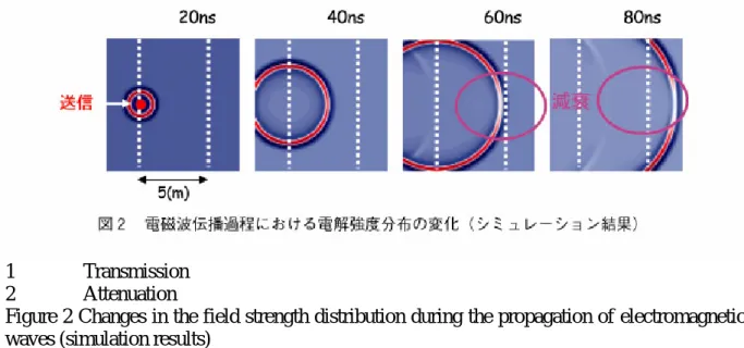
1. We simulated electromagnetic waves propagating in the underground model shown in Figure 1 according to the difference method in the time domain of Maxwell’s equations (Figure 2). Figure 2 tells that the intensity of electromagnetic waves attenuates in a place where the conductivity is high.
2. We moved the transmitting and receiving points of Figure 1 up and down respectively along the Z direction to estimate the conductivity profile. Electromagnetic waves of a shorter wavelength precisely reproduced the model’s conductivity distribution. Figure 3 shows the resulting profiles where δ = 0.5 m and λ = 0.5 to 4.0 m.
3. After completing systematic tests in all combinations of δ (0.25, 0.5, 1.0, 1.5, and 2.0 m) and λ (0.5, 0.66, 1.0, 2.0, and 4.0 m), we found that the conductivity distribution was able to be estimated with sufficient accuracy if the wavelength of electromagnetic waves used for measurement was shorter than half the parameter δ featuring a substance to be measured. 4. We believe that this method is also applicable to the evaluation of the advection velocity and distribution of a substance moving under the ground because an error occurring during the propagation of electromagnetic waves is very small if the wavelength is sufficiently shorter than the substance’s scale.
〔Utilization of the results and points to be considered〕
the propagation speed of electromagnetic waves caused by the underground structure and of the emitting and receiving properties of an antenna to be actually employed. It is also necessary to systematically conduct indoor tests to clearly find the relationship between the physical and chemical characteristics of soil, such as the concentration of a dissolved substance, and the electromagnetic properties including conductivity. Note that since the higher the frequency (the lower the wavelength), the larger the attenuation of electromagnetic waves, electromagnetic waves of an extremely short wavelength cannot be used to measure the underground conductivity.
〔Specific data〕
1 σ(y): Distribution of underground conductivity σ0: Background conductivity
σ1: Maximum conductivity in the center
2 Simulated ground containing a layer having a high concentration of electrolyte in the center (about 2.5 meq/L)
Figure 1 Conductivity distribution of an underground model used for simulation
1 Transmission 2 Attenuation
Figure 2 Changes in the field strength distribution during the propagation of electromagnetic waves (simulation results)
- 3 - True distribution at δ = 0.5 m
Estimated value at λ = 0.5 m