Modeling of Ultrasonic Guided-Wave Reflection from a Discontinuity in a Plate Structure

and Materials

Engineering

Copyright © 2013 by JSME

Modeling of Ultrasonic Guided-Wave Reflection

from a Discontinuity in a Plate Structure*

**Hitachi Research Laboratory, Hitachi, Ltd., 7-2-1 Omika-cho, Hitachi-shi, Ibaraki-ken, 319-1221, Japan

E-mail: [email protected] ***Hitachi-GE Nuclear Energy, Ltd.,

3-1-1 Saiwai-cho, Hitachi-shi, Ibaraki-ken, 317-0073, Japan

3-2-2 Saiwai-cho, Hitachi-shi, Ibaraki-ken, 317-0073, Japan

Abstract

In this paper, a combined model was proposed for reflection from a discontinuity and for a wave field of a fundamental shear horizontal guided wave in a plate structure. The reflection coefficient of a guided wave from a rectangular discontinuity can be modeled in the same way as the total reflection coefficient of a bulk wave. For the discontinuity having a slightly changed cross-sectional area, the reflection coefficient from the whole discontinuity can be calculated by spatial integration of the waves reflected from the divided regions. Some experiments and analyses were performed for 4mm-thick stainless steel plate specimens with EDM notches using a 300kHz frequency shear horizontal angle beam sensor, and for a cylindrical shell specimen (4.2m inner diameter, 9mm wall thickness) with discontinuities using a 40kHz frequency shear horizontal inter-digital sensor. The experimental reflection amplitudes were in good agreement with the analytical reflection amplitudes derived by the proposed model.

Key words

1. Introduction

The numbers of aged plants have been increasing in the power generation, oil, gas, chemical, and petro-chemical industries. A technique to efficiently evaluate integrity, especially for thickness, of many plate structures, for example pipes or tanks used in the plants, is becoming more important as present conventional non-destructive testing methods, i.e. radiographic testing, ultrasonic testing and eddy current testing, cannot meet these new inspection needs. This is because the methods naturally cover a narrow area, almost equal to their sensor size, and it is very time-consuming and cost-consuming to cover a long range or a wide area of the plate structures. Furthermore, if inspection points are placed in overhead locations, installation of scaffolds is needed before the inspection and then they must be removed afterwards; and except for radiographic testing, heat insulators must also be removed and then replaced for all inspection points.

One technique to overcome these issues is a long range inspection technique using an ultrasonic guided wave that was theoretically formulized by Gazis(1)(2). In recent years, several approaches have been proposed and some techniques have been adopted commercially(3)(4)(5)(6). In these inspection techniques, a ring sensor is used, and the discontinuity size is measured as a cross-sectional area change of the pipe by using

Yoshiaki NAGASHIMA**, Masao ENDOU**, Masahiro MIKI**,

Yoshio NONAKA*** and Ken'ichi ASAMI****

: Ultrasonic Guided Wave, Reflection Coefficient, Plate

*Received 27 Sep., 2013 (No.13-0077)

****Hitachi Power Solutions Co., Ltd.,

[DOI: 10.1299/jmmp.7.601]

amplitude of a reflected guided wave. However, the amplitude of a reflected guided wave is known to depend on the length of the discontinuity; therefore the authors previously proposed a reflection model for the guided wave in a pipe(7)(8). On the other hand, for tanks, the reflection amplitude also depends on the relative position between the sensor and the discontinuity.

Based on this background, the authors propose an analysis method to obtain the receiving gain of the guided wave. The model is based on combining the reflection from a discontinuity and a guided-wave field of a fundamental shear horizontal wave. In this paper, first, the details of the combined model are described and then the model is verified by some experiments.

2. Modeling of the guided-wave field and reflection from a discontinuity

2.1 Modeling of reflection from a discontinuity

In general, the reflection coefficient R and transmission coefficient ₀ T of an ₀ ultrasonic bulk wave from medium 1 to medium 2 are given by R₀



z₀₂z₀₁

 

/ z₀₂z₀₁



and T₀ 2z₀₂ /



z₀₂z₀₁



, respectively, where z₀₁₁c₁ is the specific acoustic impedance of medium 1 ( ₁ and c are density and velocity of medium 1) and ₁

2 2

02 c

z  is the specific acoustic impedance of medium 2 (₂and c are density and ₂ velocity of medium 2).

The reflection coefficient R and transmission coefficient T of a fundamental shear horizontal guided wave propagating in a medium of finite thickness are given by



z2 z1

 

/ z2 z1



R   and T2z₂/



z₂z₁



, respectively, where z₁₁c₁A₁ and

2 2 2

2 c A

z  are respective characteristic acoustic impedances of medium 1 and medium 2, and A and ₁ A are respective cross-sectional areas of medium 1 and medium 2 as ₂ shown in Fig. 1(a) (9). The reason why the reflection and transmission coefficients are represented by the simple equations is because the fundamental shear horizontal guided wave has same displacement through the medium and the propagation direction is parallel

even if the medium density or velocity is not changed between medium 1 and medium 2, i.e. ₁₂ and c₁c₂. If the discontinuity is a rectangular shape, the amplitude reflection coefficient is given by Eq.(1), like the total amplitude reflection coefficient of a bulk wave: (10) 2 2 1 1 2 2 2 1 1 2 cot 4 / _                z z z z z z z z R  (1)

where  2 a /, a is axial length of the discontinuity (medium 2) and  is the wavelength of the guided wave.

If the cross-sectional area of the discontinuity is slightly changed due to corrosion, for example, the reflection coefficient from the whole discontinuity is calculated by spatial integration of the waves reflected from the divided regions as shown in Fig. 1(b) and (c). Assuming that the guided wave is continuous and multiple reflection waves having over two reflection times can be ignored because of their low amplitude, the reflection wave from the whole region is given by Eq.(2):

where x is axial position, t is time, z is characteristic acoustic impedance of the _i ith small region,  is angle frequency, k is wave number and is imaginary unit.

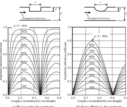
Example analysis results of two types of typical discontinuities (rectangular and semi-elliptical) are shown in Fig. 2. For the simplest rectangular discontinuity, the reflection coefficient has its maximum value when the axial length of the discontinuity is



2n1



/4

(2)

j

to the medium interface. Therefore, for guided waves, reflection occurs at a discontinuity

 

_{ }









                              N i i i i i i i m m m m m m m _{j t k x x} z z z z z z z z z z t x f 1 1 1 1 1 1 1 1 1 2 _{exp 2} 2 , 

times the wavelength ( n =1, 2‥). On the other hand, the reflection coefficient has its minimum value at n/2 times the wavelength ( n =1, 2‥). This periodicity is caused by interference between the anti-phase reflection wave from the position where the thickness is decreasing and the in-phase reflection wave from the position where the thickness is increasing. The reflection waves from the semi-elliptical discontinuity are also periodically changed for the same reason. But, its reflection coefficient decreases slightly for a long axial length. Therefore, the axial discontinuity length or shape is estimated by measuring the relationship between the frequency and reflection coefficient.

Fig. 1 Analysis models of guided-wave reflection

‥

Characteristic acoustic impedance

Zi=ρiciAi

Characteristic acoustic impedance

Zi+1=ρi+1 ci+1 Ai+1

(b) 2D analysis model Propagation direction a w d S: Cross-sectional area at the deepest part

(c) 3D analysis model

S

Characteristic acoustic impedance Z1=ρ1c1A1

Characteristic acoustic impedance Z2=ρ2c2A2

(a) Incidence, reflection and transmission of guided wave A1 : Cross section of medium 1

A2 : Cross section of medium 2

Medium 1 Medium 2 603 0.00 0.10 0.20 0.30 0.40 0.50 0.60 0.70 0.80 0.90 1.00 0 0.2 0.4 0.6 0.8 反射係数 欠陥の軸方向開口長さ（波長で規格化） 0.0 0.1 0.2 0.3 0.4 0.5 0.6 0.7 0.8 0.9 1.0 0 0.2 0.4 0.6 0.8 1 1.2 1.4 1.6 音圧反射係数 欠陥の軸方向開口長さ（波長で規格化） 系列2 系列1 系列3 系列4 系列5 系列6 系列7 系列8 系列9

Length a (normalized by wavelength)

A m p li tu d e r ef le ct io n c o ef fi c ie n t 0.0 1.0 0.8 0.6 0.4 0.2 80% d / T = 90% 70% 60% 50% 40% 30% 20% 10%

Length a (normalized by wavelength)

A m p li tu d e r ef le ct io n c o ef fi c ie n t 0.0 1.0 0.8 0.6 0.4 0.2 0.0 0.2 0.4 0.6 0.8 (b) Semi-elliptica l discontinuity (a ) Recta ngula r discontinuity

T d

T d

Propagation direction Propagation direction

a a d / T = 90% 80% 70% 60% 50% 40% 30% 20% 10% 0.0 0.2 0.4 0.6 0.8

2.2 Modeling of the wave field

For a bulk wave, the amplitude of the reflected wave changes in a complicated way if a discontinuity is located in the near-field region. Conventionally, the size of a discontinuity can be evaluated as equivalent-defect-diameter and the diameter of a circular defect shape is assumed to be a circle using the DGS (distance-gain-size) diagram (11). This concept can be used for a guided wave also.

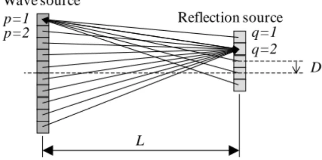
A guided wave has two characteristics. First, the amplitude of the guided wave is decreased in proportion to the square root of the distance from the source because the guided wave is a cylindrical wave. Second, the sound source is homogeneous through the wall and it can be treated as a line source on a two-dimensional plane as shown in Fig. 3. Therefore, the reflected wave received by the wave source (a transducer) is calculated by the Kirchhoff method using the following procedure. First, the vibration of element q on the discontinuity is expressed by Eq.(3)

(3)

where r r₁r₀ ,

r

₀ is the position vector of element p on the wave source,

r

₁ is the position vector of element q on the reflection source,  is angular frequency, t is time, is imaginary unit, and k is wave number. Next, the vibration xp

 

t of element

p on the wave source (transducer) is expressed by Eq.(4)

 



_

  





q q p y t jkr r t x exp ' ' 1 (4)

where r'r₂r₁ , and r₂ is the position vector of element p. Finally, the amplitude C

of the reflected wave received by the wave source is expressed by Eq.(5).



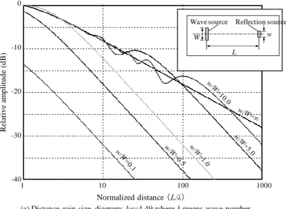
 p p x C 2 (5)

When the reflection source is in front of the wave source, the DGS diagram of the guided wave that has ka =4.49（ k is wave number and a is the half length of the sound source）is shown in Fig. 4(a). In the figure, the horizontal axis is normalized distance (distance L is normalized by wavelength ), and the vertical axis is relative amplitude normalized by the amplitude of the reflected wave from the reflection source =∞ ( w is width of the reflection source and is width of the wave source) at the normalized distance = 1. The amplitude from the reflection source =∞ decreases 10dB for each power of ten change in distance, but the amplitude from the finite width of the reflection source decreases 20dB for each power of ten change in distance at the far-field, and the relative amplitude is proportional to the width of the reflection source. The relationship between the normalized lateral distance D/ and relative amplitude at

100 / L is shown in Fig. 4(b). L Wave source Reflection source p=2 q=1 q=2 p=1 D

Fig. 3 Analysis model of guided-wave field

j W w / W W w /

 



_







p p q j t kr r A t y exp 

Fig. 4 Analysis results of relative amplitude from several size discontinuities by the wave field model

3. Experiments

3.1 Experiment with plate specimens

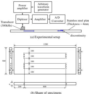
In order to measure amplitude of the reflected wave from rectangular discontinuities, 2 types of stainless steel plate specimens (thickness = 4mm) with artificial discontinuities were fabricated. One type specimen had 4 discontinuities with width of 100mm and height of h =0.5mm to h =2.0mm in steps of 0.5mm (Fig. 5(b)). The other type specimen had 2 discontinuities with width of 100mm and each height of h =2.5mm or h =3.0mm.

A block diagram of the experimental system is shown in Fig. 5(a). An arbitrary function generator, power amplifier, diplexer receiver amplifier and A/D converter (maximum sampling rate = 1GS/s, vertical resolution = 8 bits) configured the system. The transducer was a shear-vibration type with a resonance frequency of 300kHz. It was bonded on an acrylic wedge with a refraction angle of 90deg which matched the shear horizontal wave velocity.

The transducer was placed on a plate specimen using viscosity medium coupling, opposite the fabricated discontinuities, and a normal load was given until the amplitude

1 10 100 1000 Normalized distance （L/λ） 0 -10 -20 -30 -40 Re la ti v e am p li tu d e (d B) L W w

Wave source Reflection source

(b) Relationship between lateral distance and amplitude: ka=4.49, L/λ=100.

0 -10 -20 -30 -40 Re la ti v e am p li tu d e (d B) Normalized distance （D/λ） -30 -20 -10 0 10 20 30 w/W=1.0 w/W=0.5 w/W=5.0 w/W=10.0 w/W=∞ D W w

Wave source Reflection source

L=100λ

(a) Distance-gain-size diagram: ka=4.49 where k means wave number and a means half length of wave source

became stable. Then, the transducer was placed 700mm from the discontinuities, and the reflected wave was recorded. The amplitude of the reflected wave from the plate end was also measured. In the experiments, the transducer was driven by a 300kHz tone-burst wave.

The amplitude reflection coefficients of rectangular discontinuities obtained from the experiment with the plate specimens are shown in Fig. 6. The filled circles are experimental results normalized by the reflection amplitude of the through-thickness discontinuity with width of 100mm. Solid lines are theoretical results obtained by Eq.(1). In this experiment, the frequency of the guided wave was 300kHz and the length of the rectangular discontinuity was 1mm, then the length of the discontinuity normalized by the wavelength (~10.5mm) was about 0.1. In this figure, experimental results are plotted between analytical values of 1.0mm length discontinuity and 1.5mm length discontinuity. Nominal length of the discontinuity was 1mm, and the results obtained for the proposed model were approximately in agreement with the experimental results.

Power amplifier

Arbitrary waveform generator

Stainless steel plate (Thickness = 4mm) Diplexer Amplifier Transducer (300kHz) discontinuity A/D Converter (b) Shape of specimens (a) Experimental setup

h3 h4 1200 100 100 100 100 100 h2 h1 500 800 4 200

3.2 Experiment with the cylindrical shell specimen

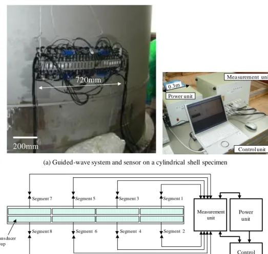
The guided-wave system and sensor are shown in Fig. 7(a). The system included arbitrary function generators, power amplifiers, an A/D converter and a computer for control. The sensor had 8 inter-digital transducer groups (4 x 2 rows). The inter-digital transducers had a shear mode element and the fundamental shear horizontal mode guided wave with no dispersion was excited.

In order to control the transmission direction, 4 pairs of transducers were set on the cylindrical shell specimen with a separation of 20mm (Fig. 7(b)), which is about one-quarter of the wavelength of the 40kHz shear horizontal mode, and a one-quarter period delayed waveform was applied to each pair. Backward transmission was actively suppressed by the inter-digital transducers according to the following principle. A synthetic traveling wave in the plus (right hand) direction A

 

x,t and a synthetic traveling wave in the minus (left hand) direction A

 

x,t are given by Eqs.(6) and (7), respectively:

(6)

(7) where x is the axial coordinate of the pipe, A and ₁ A are amplitudes of the ₂ transmitting wave of positions 1 and 2, respectively,  is angle frequency, t is time, k is wave number, T



2/



is period, 



2/k



is wavelength, and is imaginary unit. For A₁A₂ in Eqs.(6) and (7), a synthetic wave traveling in the plus direction is doubly super-positioned, and a synthetic wave traveling in the minus direction is suppressed to zero. This is shown in Fig. 8.

In practice, the transmitting signals used for inspection are not continuous waves but burst waves that have a limited duration. Then, the waveform applied to the front row of the transducer pairs was the inverse of the waveform applied to the rear row and it had a one-quarter period delay. In this method, the amplitude of the synthetic traveling wave in the plus direction could not be completely doubled, but the amplitude of the synthetic traveling wave in the minus direction could be completely decreased to zero in theory. For inspection, distinguishing between the reflection wave from one direction (signal) and the Fig. 6 Amplitude reflection coefficients of rectangular discontinuities on plate specimens (frequency =

300kHz): experimental values are normalized by signal amplitude of through-thickness discontinuity

j 607 0.0 0.1 0.2 0.3 0.4 0.5 0.6 0.7 0.8 0.9 1.0 0.0 0.1 0.2 0.3 0.4 0.5 0.6 0.7 0.8 0.9 1.0 音圧反射係数 矩形欠陥深さ（肉厚比） discontinuity depth (%) A m pl it ud e re fl ec ti on c oe ff ic ie nt 30 0 10 20 40 50 60 70 80 90 100 0.5mm (0.05) 1.0mm (0.1) 1.5mm(0.14) 2.0mm (0.19) a=2.5mm (a/ λ = 0.24) 1.0 0.0 0.2 0.4 0.6 0.8

 

 _  _  _ __  _  _{ } 4 4 2 1 ,    k x T t j kx t j e A e A t x A

 

 _  _  _ _ _  _  _{ } 4 4 2 1 ,    k x T t j kx t j e A e A t x A

reflection wave from another direction (noise or false signal) is important. Therefore, almost the same processing was performed for received signals.

Measurement unit Power unit Control unit

(a) Guided-wave system and sensor on a cylindrical shell specimen

(b) System configuration

Co-a xia l ca bles

Segment 1 Segment 3 Segment 5 Segment 7 Segment 2 Segment 4 Segment 6 Segment 8 720mm 200mm Power unit

Mea surement unit

Control unit

Transducer group

Fig. 7 Photo of the guided-wave system and sensor and a block diagram of the system

Rea r group Front group super-positioned Suppressed 1/4λ Time Time Tra nsmission signa l (rea r)

Tra nsmission signa l (front) 1/4T A m p li tu d e A m p li tu d e

Fig. 8 Transmission direction control by the inter-digital transducers

A cylindrical shell specimen was used as shown in Fig. 9. The specimen was SUS304, with 4200mm inner diameter, 2800mm height, and 9mm nominal wall thickness. Two axial butt welds were positioned, one at 0deg and the other at 180deg. Three different shapes of artificial discontinuities (O, A, R) were fabricated on the inner diameter (ID) side of the specimen. The guided-wave sensor was positioned at 6 locations (P1 to P6), and the guided

wave was transmitted in the direction indicated by the arrows. The reflection signal amplitude from the discontinuity was measured at several frequencies.

Fig. 9 Cylindrical shell specimen and artificial discontinuities

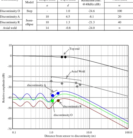
The relative reflection amplitudes of the discontinuities obtained from the experiment with the cylindrical shell specimen are shown in Fig. 10. Filled marks are experimental results. Solid lines are analytical amplitudes obtained by Eq.(1) or Eq.(2), and Eq.(5). For comparison of the experimental amplitudes and the analytical amplitudes, the experimental amplitudes were corrected by using the ratio between the analytical amplitude of =∞ and an experimental amplitude of the top end of the cylindrical shell.

In the reflection coefficient analysis, sizes of discontinuities were precisely measured by the replica method, and were modeled by the values of Table 1. For example, discontinuity O, 100mm square length and 1mm depth, was approximately modeled as a 1mm-step discontinuity, because reflection waves at the decreasing step and increasing step hardly interfere with each other since the difference of propagation distance was 200mm and the duration time of waveform was about 3 cycles as shown in Fig. 8. Discontinuities A and R were modeled as a semi-elliptical shape, with depths of 6.5mm and 1.27mm, respectively, and width of 10mm. Axial weld, i.e. excess weld metal, was also modeled as a semi-elliptical shape, with length of 14mm and depth of -0.8mm, where the minus value means thickness was increasing.

Widths of the discontinuities for the wave field analysis were modeled by the values of Table 1. The width w of discontinuity A, a pair of 10mm-diameter drilled holes, was modeled as 20mm. Width of the axial weld was defined as ∞. The guided-wave sensor was modeled as =720mm width, 40kHz frequency. The solid lines in Fig. 10 were calculated by this wave field analysis, and the values were corrected by the reflection coefficients in Table 1.

In Fig. 10, the relative amplitudes of discontinuities were in good agreement with

2800 1560 4266 800 1000 3626 discontinuity A discontinuity O P2 P3 P1

(a) Positions of discontinuities and positions of the sensor (P1 to P6) on cylindrical shell specimen

800 1100 900 P4 P5 P6 480 900 500 (mm) discontinuity R 40 9 1.3 discontinuity A (S=131㎜2₎ discontinuity O (S=100㎜2_{) discontinuity R (S=40㎜}2₎ 10 100.5 100.7 1 9 9 φ10.2 15 6.5 φ10.1 ID OD ID OD ID OD (b) Discontinuity shapes Weld Weld Weld 0 deg 180 deg -180 deg W w / W 609

analytical values, and the proposed model was verified. By using the model, detectable discontinuities were estimated by providing their shape and size, and in the future, it is expected that the shape and size can be estimated using the amplitude of received signals with multiple frequency transmissions.

Table 1 Reflection coefficients of discontinuities

Discontinuity

Reflection model Wave field model Model Length (mm) Depth (mm) Reflection coef.

@40kHz (dB) Width (mm) a d w Discontinuity O Step - 1.0 -24.6 100 Discontinuity A Semi-ellipse 10 6.5 -8.1 20 Discontinuity R 10 1.3 -21.3 40 Axial weld 14 -0.8 -24.0 ∞

4. Conclusions

A combined model for reflection from a discontinuity and for the guided-wave field of the fundamental shear horizontal guided wave in a plate structure was proposed. Some experiments and analyses were performed for 4mm-thick stainless steel plate specimens and for a cylindrical shell specimen with an inner diameter of 4.2m and wall thickness of 9mm. It was found that reflection coefficient of the guided wave from a rectangular discontinuity could be modeled in the same way as the total reflection coefficient of a bulk wave. For a discontinuity having a cross-sectional area that slightly changed, the reflection coefficient from the whole discontinuity could be calculated by spatial integration of the waves reflected from the divided regions. The experimental results were in good agreement with the analytical values obtained using the proposed combined model.

Fig. 10 Relative signal amplitude of discontinuities of the cylindrical shell specimen (frequency = 40kHz): experimental results and analytical results obtained by the proposed model

-70.0 -60.0 -50.0 -40.0 -30.0 -20.0 -10.0 0.0 10.0 0.1 1.0 10.0 100.0 相対エ コ ー 高さ (d B ) センサから欠陥までの距離（m）

Dista nce from sensor to discontinuity (m)

R e la ti v e a m p li tu d e ( d B ) 0 -10 -20 -30 -40 -50 -60 -70 10 discontinuity O 0.1 1.0 10.0 100.0 discontinuity R Top end discontinuity A Axia l Weld

(1) Gazis, D.C., Three-Dimensional Investigation of the Propagation of Waves in Hollow Circular Cylinders. I. Analytical Foundation, Journal of Acoustical Society of America, Vol.31, No.5 (1959), pp.568-573.

(2) Gazis, D.C, Three-Dimensional Investigation of the Propagation of Waves in Hollow Circular Cylinders. II. Numerical Results, Journal of Acoustical Society of America, Vol.31, No.5 (1959), pp.573-578.

(3) Mudge, P. J., Field Application of the Teletest Long-range Ultrasonic Testing Technique, Insight, Vol.43, No.2 (2001), pp.74-77.

(4) Sheard, M. and McNulty, A., Field Experience of Using Long-range Ultrasonic Testing, Insight, Vol.43, No.2 (2001), pp.79-83.

(5) Li, J. and Rose J. L., Angular-Profile Tuning of Guided Waves in Hollow Cylinders Using a Circumferential Phased Array, IEEE Transactions on Ultrasonic, Ferroelectrics and Frequency Control, Vol.49, No.12 (2002), pp.1720-1729.

(6) Rose, J. L., Sun, Z., Mudge, P. J. and Avioli, M. J., Guided Wave Flexural Mode Tuning and Focusing for Pipe Testing, Materials Evaluation, Vol.61, No.2 (2003), pp.162-167. (7) Nagashima, Y., Endou, M. and Kouga, I., Discontinuity-length Sizing Potential Using

Ultrasonic Guided Waves in Pipes, Proceedings of 15th International Conference on Nuclear Engineering, (2007), ICONE15-10637

(8) Nagashima, Y., Endou, M., Miki, M., Odakura, M. and Maniwa, K., Defect Sizing Method Using Ultrasonic Guided Waves in Pipes, Review of Progress in Quantitative Nondestructive Evaluation, Vol.28 (2008), pp.1583-1590

(9) Tomikawa, Y., Ultrasonic electronics vibration theory (in Japanese), (1998) pp.5-6, Asakura Publishing, Co., Ltd.

(10) American Society for Nondestructive testing, Nondestructive testing handbook third edition, volume 7, Ultrasonic testing, (2007), p.372

(11) Kimura, K. and Matsumoto, S., DGS Diagrams for Angle Probes, 3rd European Conference on NDT Florence, Vol. 3, (1984), pp. 93-102

References