Optimization-Based Iterative Methods for Solving Nonlinear Complementarity Problems(Nonlinear Analysis and Mathematical Economics)

Optimization-Based

Iterative

Methods

for Solving

Nonlinear

Complementarity

Problems

TAJI

Kouichi

(

田地宏一

)

FUKUSHIMA Masao

(

福島雅夫

)

IBARAKI

Toshihide

(

茨木俊秀

)

Department of Applied Mathematics and

Physics,

Faculty

of

Engineering,

Kyoto

University, Kyoto

606,

JAPAN

1

Introduction

We consider the nonlinear complementarity problem, which is to find a vector $x\in R^{n}$

such that

$x\geq 0,$$F(x)\geq 0$ and $x^{T}F(x)=0$, (1)

where $F(x)=(F_{1}(x), F_{2}(x),$ _$\ldots,$$F_{n}(x))^{T}$ is a given continuously differentiable mapping

from $R^{n}$ intoitself and $T$ denotes transposition. This problemhas been used toformulate

and study various equilibrium problems including the traffic equilibrium problem, the spatial economic equilibrium problem and Nash equilibrium problem [4, 12, 16].

Thenonlinear complementarity problem (1) isa specialcaseof the variational inequality problem, which is tofind a vector $x^{*}\in S$ such that

$(x-x^{*})^{T}F(x^{*})\geq 0$ for _瓠1 $x\in S$

,

(2)

where $S$ is a nonempty closed convex set in $R^{n}$

.

Problem (1) corresponds to the case $S=R_{+}^{n}$, the nonnegative orthant of$R^{n}$

.

The variational inequalityproblemhas also been

used to formulate and study various equilibrium problems arisingin economics, operations research, transportation and regional sciences.

To solve thenonlinear complementarityproblem (1) andthe variationalinequality prob-lem (2), various iterative algorithms, such as fixed point algorithms, projection methods,

nonlinear Jacobi method, successive over-relaxation methods and Newton method, have

in the proof that the problem has a solution. Fixed point algorithms are useless for prac-tical computations becausetheir

convergence

are extremelyslow [14]. The other methods

are generalizations of methods for systems of nonlinear equations and their convergence

results have been obtained $[7, 13]$

.

But, in general, these methods do not have globally

convergent property.

Assuming the monotonicity of mapping $F$, Fukushima [5] has recently proposed a

dif-ferentiable optimization formulation for variational inequality problem (2) and proposed

a decent algorithm to solve (2). Based on this optimization formulation, Taji et al. [15] proposed a modification of Newton method for solving the variational inequality problem

(2), and proved that, under the strong monotonicity assumption, the method is globally and quadratically convergent.

In this paper we apply the methods of Fukushima [5] and Taji et al. [15] to the

non-linear complementarity problem. We show that those specialized methods can take full

advantage of the special structure of problem (1), thereby yielding new globally

conver-gent algorithms for solving monotone complementarity problems. We remark that the

constraint set of nonlinear complementarity problem is $R_{+}^{n}$ which is clearly not

com-pact, while the descent method by Fukushima [5] has assumed that the constraint set is

compact. In this paper we show that the compactness assumption can be removed for

the nonlinear complementarity problem. We also present some computational results to

demonstrate that those methods are practically efficient.

2

Equivalent

optimization

problem

Wefirstreview the results obtainedbyFukushima [5]for thegeneralvariational inequal-ity problem (2). Let $G$ be an _$nxn$ symmetric positive definite matrix. The projection under the G-norm of$x\in R^{n}$ onto the closed convex set $S$, denoted Proj_$s,c(x)$, is defined as the unique solution of the following

mathematical

program:

minimize $||y-x||_{G}$ subject to $y\in S$,

where $||\cdot||_{G}$ denotes the G-norm in $R^{n}$, which is defined by

11

$x||_{G}=(x^{T}Gx)^{\frac{1}{2}}$.

Using this notation, we define function $f$ : $R^{n}arrow R$ by

$f(x)= \max\{-(y-x)^{T}F(x)-\frac{1}{2}(y-x)^{T}G(y-x)|y\in S\}$ ₍₃₎

$=-(H(x)-x)^{T}F(x)- \frac{1}{2}(H(x)-x)^{T}G(H(x)-x)$

,

₍₄₎

where the mapping $H:R^{n}arrow R^{n}$ is defined by

It can be shown [5] that the function $f$ is continuouslydifferentiable whenever so is the mapping $F$, and its gradient is given by

$\nabla f(x)=F(x)-[\nabla F(x)-G](H(x)-x)$

.

(6)

The function $f$ has the property that $f(x)\geq 0$ for $aUx\in S$ and $f(x)=0$ whenever $x$ is a solution to the variational inequality problem (2). Hence problem (2) is equivalent

to the followingoptimization problem:

minimize $f(x)$ subject to $x\in S$

.

(7)

In addition, when $\nabla F(x)$ is positive definite for all $x\in S$, it can be shown that, if $x\in S$ is a stationary point of problem (7), i.e.,

$(y-x)^{T}\nabla f(x)\geq 0$ for all $y\in S$, (8)

then $x$ is a global optimal solution of problem (7), and hence it solves the nonlinear

complementarity problem (1).

Let us now specialize the above results to the complementarity problem. For general

variational inequality problems, it may be expensive to evaluate the function $f$ unless $S$

is tractable. In the case of the complementarity problem (1), the set $S$ turns out to be

$R_{+}^{n}$. So, if we in particular let $G$ be a diagonal matrix $D=diag(\delta_{1}, \ldots, \delta_{n})$, where $\delta_{:}$ are

positive constants, then the mapping $H$ takes the explicit form

$H(x)= \max(0, x-D^{-1}F(x))$ (9)

where maximum operator is taken component-wise, i.e.

$H_{i}(x)= \max(0, x_{i}-\delta_{i}^{-1}F_{i}(x))$, $i=1,$

$\ldots,$$n$

.

(10)

Hence the function $f$ and its gradient can be represented as

$f(x)= \frac{1}{2}F(x)^{T}D^{-1}F(x)-\frac{1}{2}\max(0, D^{-1}F(x)-x)^{T}D\max(0, D^{-1}F(x)-x)$

$= \sum_{=1}^{n}\frac{1}{2\delta_{1}}\{F_{i}(x)^{2}-(\max(0, F_{1}(x)-\delta_{i}x_{i}))^{2}\}$ , (11)

and

$\nabla f(x)=\nabla F(x)D^{-1}F(x)+(I-\nabla F(x)D^{-1})\max(0, F(x)-Dx)$ (12)

respectively, and the optimization problem (7) becomes

minimize $f(x)$ subject to $x\geq 0$

.

(13)

In this special case, it is therefore straight forward to evaluate the function $f$ and its gradient. Furthermore, the optimization problem (13) has a simple constraint.

3

Descent

methods

In this section, we specialize the methods of Fukushima [5] and Taji et al. [15], which

wereoriginally proposed for variationalinequality problems, to the nonlinear

complemen-tarity problem (1). Throughout this section, we let $D$ be a positive definite diagonal

matrix and the function $f$ be defined by (11). We $al$so suppose that the mapping $F$ is

strongly monotone on $R_{+}^{n}$ with modulus $\mu>0$ i.e.,

$(x-y)^{T}(F(x)-F(y))\geq\mu||x-y||^{2}$ _{for all} $x,$$y\geq 0$

.

(14) The first method uses the vector

$d=$ $H(x)-x$

$= \max(0, x-D^{-1}F(x))-x$ (15)

as a search direction at $x$

.

When the mapping $F$ is strongly monotone with modulus $\mu$,

it is shown [5] that the vector $d$given by (15) satisfies the descent condition

$d^{T}\nabla f(x)\leq-\mu||d||^{2}$

Thus the direction $d$ can be used to determine the next iterate by using the following

Armijo-type line search rule: Let $\alpha$ $:=\beta^{\dot{m}}$, where $\hat{m}$ is the smallest nonnegative integer

$m$ such that

$f(x)-f(x+\beta^{m}d)\geq\sigma\beta^{m}||d||^{2}$,

where $0<\beta<1$ and $0<\sigma$

.

Algorithm

1

a:

choose $x^{0}\geq 0,$ $\beta\in(0,1)$, $\sigma>0$ and a positive diagonal matrix $D$; $k$ $:=0$

while

convergence

criterion is not satisfied do

$d^{k}$ _{$:= \max(0, x^{k}-D^{-1}F(x^{k}))-x^{k}$}; $m$ $:=0$ while $f(x^{k})-f(x^{k}+\beta^{m}d^{k})<\sigma\beta^{m}||d^{k}||^{2}$ do $m$ $:=m+1$ endwhile $x^{k+1}$ $:=x^{k}+\beta^{m}d^{k}$ ; $k$ $:=k+1$ endwhile

In line searchprocedure of this algorithm, we examine only thepoints shorter than unit

step size. But weexpect todecrease the value of the function $f$ when the longer step size

is chosen. Therefore we propose the algorithmin which we modify Algorithm la so that

the longer step size can be selected.

Algorithm

1

$b$

:

choose $x^{0}\geq 0$, $\beta_{1}>1$, $\beta_{2}\in(0,1)$, $\sigma>0$ and a positive diagonal matrix$D$; $k$ $:=0$

while convergence criterion is not satisfied do

$d^{k}$ _{$:= \max(0, x^{k}-D^{-1}F(x^{k}))-x^{k}$};

$\hat{t}$

$:= \max\{t|x^{k}+td^{k}\geq 0, t\geq 0\}$;

$m$ $:=0$

if $f(x^{k})-f(x^{k}+d^{k})\geq\sigma||d^{k}||^{2}$ then

while $\beta_{1}^{m}\leq\hat{t}$ and $f(x^{k})-f(x^{k}+\beta_{1}^{m}d^{k})\geq\sigma\beta_{1}^{m}||d^{k}||^{2}$

and $f(x^{k}+\beta_{1}^{m+1}d^{k})\leq f(x^{k}+\beta_{1}^{m}d^{k})$ do $m$ $:=m+1$ endwhile $x^{k+1}$ $:=x^{k}+\beta_{1}^{m}d^{k}$ else while $f(x^{k})-f(x^{k}+\beta_{2}^{m}d^{k})<\sigma\beta_{2}^{m}||d^{k}||^{2}$ do $m$ $:=m+1$ endwhile $x^{k+1}$ $:=x^{k}+\beta_{2}^{m}d^{k}$ endif $k$ $:=k+1$ endwhile

Note that, since an evaluation of $f$ at a given point $x$ is equivalent to evaluating the

vector$\max(O, x-D^{-1}F(x))$, the

vector

$H(x^{k})= \max(0, x^{k}-D^{-1}F(x^{k}))$ has already been

found at the previous iteration

as

a by-product of evaluating $f(x^{k}+\beta^{m}d^{k})$

.

Therefore

one need not compute the search direction $d^{k}$ at the beginning ofeach iteration.

In the descent method proposed by Fukushima, to prove that the method is globally

convergent it is necessary not only the st$r$ong monotonicity ofmapping but the

compact-ness of constraint set. However, in the case of nonlinear complementarity problem, we

can prove that Algorithms la and lb

convergence

globally ifonly $F$ is strongly monotone.

Proposition 3.1

_If

$F$ is strongly monotone on $R_{+}^{n}$, then

$\lim$ _{$f(x)=+\infty$}

.

Proof. For convenience, we define

$f_{i}(x)=F_{i}(x)^{2}-( \max(0, F_{i}(x)-\delta_{i}x_{i}))^{2}$, (16)

hence $f$ is written as $f(x)= \sum_{=1}^{n}\frac{1}{2\delta_{i}}f_{i}(x)$

.

We first show that $f_{i}(x)\geq 0$ for all $x\geq 0$

.

If $F_{i}(x)-\delta_{i}x_{i}\leq 0$, then $f_{i}(x)=F_{1}(x)^{2}\geq 0$

.

So we consider the case $F_{i}(x)-\delta_{i}x_{i}>0$

.

Since

$6_{i}>0,$ $x_{i}\geq 0$ and $F_{i}(x)>\delta_{*}x$; hold, we see, from (16), $f_{t}(x)$ $=$ $F_{i}(x)^{2}-(F_{1}(x)-\delta_{i}x_{i})^{2}$

$=$ $\delta_{i}x_{i}(2F_{1}(x)-\delta_{i}x_{i})$

$\geq$ $(\delta_{i}x_{i})^{2}$ $\geq$ $0$

.

Let $\{x^{k}\}$ be a sequence such that $x^{k}\geq 0$ and

Il

$x^{k}||arrow\infty$

.

Taking a subsequence, if

necessary, there exists a set $I\subset\{1,2, \ldots, n\}$ such that $x_{i}^{k}arrow+\infty$ for $i\in I$ and $\{x_{i}^{k}\}$ is

bounded for $i\not\in I$. Without loss of generality, $\{x^{k}\}$ itself has a such set $I$. From $\{x^{k}\}$,

we define a sequence $\{y^{k}\}$ where $y_{i}^{k}=0$ if $i\in I$ and $y_{i^{k}}=x_{i}^{k}$ if $i\not\in I$. From (14) and the

definition of $y^{k}$, we have

$\sum_{i\in I}(F_{1}(x^{k})-F_{1}(y^{k}))x^{\dot{k}}\geq\mu\sum_{:\in I}x^{k^{2}}$

By Cauchy’s inequality

$||F(x^{k})-F(y^{k})$ $||||$ $x^{k}-y^{k}||\geq(F(x^{k})-F(y^{k}))^{T}(x^{k}-y^{k})$,

we have

$( \sum_{i\in I}(F_{i}(x^{k})-F_{1}(y^{k}))^{2})^{\frac{1}{2}}(\sum_{i\in I}x^{k^{2}})^{\frac{1}{2}}\geq\sum_{i\in I}(F_{1}(x^{k})-F_{i}(y^{k}))x^{k}$,

hence we have

$\sum_{:\in I}(F_{i}(x^{k})-F_{i}(y^{k}))^{2}\geq\mu^{2}\sum_{i\in I}x_{i}^{k^{2}}$ (17)

Since, fromthe definition of $y^{k},$ $\{y^{k}\}$ is bounded, $\{F_{i}(y^{k})\}are$ also bounded for all $i$, and

$x^{k};arrow+\infty$ for all $i\in I,$ (17) implies

As shown at the beginning of the proof, $f_{1}(x)=F_{i}(x)^{2}\geq 0$ if $F_{i}(x)-\delta_{i}x_{i}\leq 0$, and

$f(x^{k})\geq(\delta_{i}x_{i})^{2}$ if $F_{1}(x)-\delta_{i}x_{i}>0$

.

Therefore we have

$f(x^{k})$ $= \sum_{=1}^{n}\frac{1}{2\delta_{i}}f_{1}(x)$

$\geq$ $\sum_{i\in I}\frac{1}{2\delta_{1}}f_{i}(x)$

$\geq$ $\sum_{:\in I}\frac{1}{2\delta_{*}}\min(F_{1}(x)^{2}, (\delta_{i}x.)^{2})$

.

Since $x_{1}^{k}arrow+\infty$ for all $i\in I$ and

$\sum_{i\in I}F_{1}(x^{k})^{2}arrow\infty$, it follows that $f(x^{k})arrow+\infty$

.

$\square$

Theorem 3.1 Suppose that the mapping $F$ is continuously

differentiable

and strongly

monotone with modulus $\mu$ on $R_{+}^{n}$

.

Suppose also that $\nabla F$ is Lipschitz continuous on any

bounded subset

_of

$R_{+}^{n}$

.

Then,

for

any starting point $x^{0}\geq 0$, the

sequence

$\{x^{k}\}$ generated

by Algorithm la or Algorithm $lb$ converges to the unique solution

of

problem (1)

if

the

positive constant $\sigma$ is chosen to be

suff

ciently small such that _$\sigma<\mu$

.

Proof. By proposition 3.1, the level set $S=\{x|f(x)\leq f(x^{0})\}$ is shown to be bounded.

Hence $\nabla F$ is Lipschitz continuous on $S$

.

Since $F$is continuously differentiable it is easy to show that $F$ is also Lipschitz continuous on $S$

.

Under these conditions, it is not difficult

to show that $\nabla f$ is Lipschitz continuous on $S$, i.e., there exists a constant $L>0$ such

that

$||\nabla f(x)-\nabla f(y)||\leq L||x-y||$ for all $x,$$y\in S$

.

The remainder of this proof is the same as the proofof [5, theorem4.2]. $\square$

The second method is a modification of Newton method, which incorporates the line

search strategy. The original Newton method for solving the nonlinear complementarity

problem (1) generates a sequence $\{x^{k}\}$ such that $x^{0}\geq 0$ and $x^{k+1}$ is determined as

$x^{k+1}$ $:=\overline{x}$, where $\overline{x}$ is a solution to the following linearized complementarity problem:

$x\geq 0,$$F(x^{k})+\nabla F(x^{k})^{T}(x-x^{k})\geq 0$ and $x^{T}(F(x^{k})+\nabla F(x^{k})^{T}(x-x^{k}))=0$

.

(18)

It is shown [13] that, under suitableassumptions, the sequencegenerated by (18) quadrat-ically converges to a solution $x^{*}$ of the problem (1), provided that the starting point $x^{0}$

is chosen sufficiently close to $x^{*}$

.

Taji et al. [15] have shown that, when the mapping

$F$ is strongly monotone with modulus $\mu$, the vector

$d:=\overline{x}-x^{k}$ obtained by solving the

linearized complementarity problem (18) satisfies the inequality

Therefore, $d$ is actually a feasible descent direction of $f$ at $x^{k}$, if the matrix _$D$ is chosen

to satisfy $||D||= \max_{i}(\delta_{1})<2\mu$

.

Using this result, we can construct a modified Newton

method for solving the nonlinear complementarity problem (1).

Algorithm 2:

choose $x^{0}\geq 0$, $\beta\in(0,1)$, $\gamma\in(0,1)$, $\sigma\in(0,1)$and a positive diagonal matrix $D$;

$k$ $:=0$

while

convergence

criterion is not satisfied do

find hi such that

$x\geq 0,$$F(x^{k})+\nabla F(x^{k})^{T}(x-x^{k})\geq 0$ and $x^{T}(F(x^{k})+\nabla F(x^{k})^{T}(x-x^{k}))=0$;

$d^{k}$ $:=\overline{x}-x^{k}$ if$f(x^{k}+d^{k})\leq\gamma f(x^{k})$ then $\alpha_{k}$ $:=1$ else $m$ $:=0$ while $f(x^{k})-f(x^{k}+\beta^{m}d^{k})<-\sigma\beta^{m}d^{k^{T}}\nabla f(x^{k})$ do $m$ $:=m+1$ endwhile $\alpha_{k}$ $:=\beta^{m}$ endif $x^{k+1}$ $:=x^{k}+\alpha_{k}d^{k}$ ; $k$ $:=k+1$ endwhile

By applying the results proved in [15] for the general variational inequality problem, we

see that, when the mapping $F$ is strongly monotone with modulus $\mu$, this algorithm is

convergent to the solution of (1) for any $x^{0}\geq 0$ if the matrix $D$ is chosen such that

$||D||= \max(\delta_{i})<2\mu$

.

From [15], we also see that the rate ofconvergence is quadratic if $\nabla F$ is Lipschitz continuous on a neighborhood of the unique solution $x^{*}$ of problem (1)

and the strict complementarity condition holds at $x^{*}i.e.,$ $x^{*}=0$ implies $F_{i}(x^{*})>0$ for

all $i=1,2,$$\ldots,$$n$.

4

Computational results

In this section, we report some numerical results for Algorithms la, lb and 2 discussed

in the previous section. All computer programs were coded in FORTRAN and the runs

Throughout the $co$mputational experiments, the parameters used in algorithms were

set as $\beta=\beta_{1}=\beta_{2}=0.5,$ $\gamma=0.5$ and $\sigma=0.0001$

.

The positive diagonal matrix $D$ was

chosen to be the identity matrix multiplied by a positive parameter $\delta>0$

.

Therefore the merit function (11) can be written more simply as

$f(x)= \frac{1}{2\delta}\sum_{i=1}^{n}\{F_{1}(x)^{2}-(\max(0^{\cdot}, F_{1}(x)-\delta x_{i}))^{2}\}$

.

(19)

The search direction ofAlgorithms la and lb can also be written as

$d^{k}$

$:= \max(0,$$x^{k}- \frac{1}{\delta}F(x^{k}))-x^{k}$

.

The convergence criterion was

$| \min(x;, F_{i}(x))|\leq 10^{-5}$ for all $i=1,2,$

$\ldots,$$n$

.

(20)

For comparison purposes, we also testedtwopopular methods for solvingthe nonlinear

complementarity problem, the projection method [3] and the Newton method without

line

search [9]. The projection method generates a sequence $\{x^{k}\}$ such that $x^{0}\geq 0$ and

$x^{k+1}$ is determined from $x^{k}$ by

$x^{k+1}$ _{$:= \max(0,$}$x^{k}- \frac{1}{\delta}F(x^{k}))$ , (21)

for all $k$

.

Note that this method may beconsidered afixedstep-size variant ofAlgorithms

la and lb. When the mapping $F$ is strongly monotone and Lipschitz continuous with

constants $\mu$ and $L$, respectively, this method is globally convergent if

6

is chosen large

enough to satisfy $\delta>L^{2}/2\mu$ (see [13, Corollary 2.11.]).

The mappings used in our numerical experiments are of the form

$F(x)=Ix+\rho(N-N^{T})x+\phi(x)+c$_, (22)

where $I$ is the _$nxn$ identity matrix, $N$ is an _$nxn$ matrix such that each row contains

only one

nonzero

element, and $\phi(x)$ is a nonlinear monotone mapping with components

$\phi_{i}(x_{i})=p_{i}x_{i}^{4}$, where $p$; are positive constants. Elements of matrix $N$ and vector $c$ as

well as coefficients $p_{i}$ are randomly generated such that $-5\leq N_{*j}\leq 5,$ $-25\leq c_{t}\leq 25$

and 0.001 $\leq p;\leq 0.006$

.

The results are shown in Tables $1\sim 4$

.

All starting points

were chosen to be $(0,0, \ldots, 0)$

.

In the tables, $\# f$ is the total number of evaluating the

merit function $f$ and all CPU times are in seconds and exclude input/output times. The

parameter $\rho$ is used to change the degree of asymmetry of $F$, namely $F$ deviates from

symmetry

as

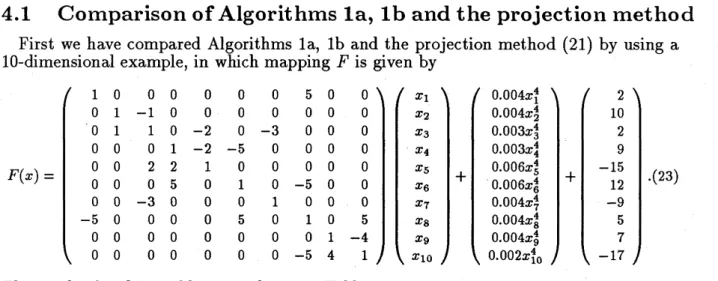
$\rho$becomes large. Since the matrix $I+\rho(N-N^{T})$ is positivedefinite for any $\rho$ and $\phi_{1}(x_{i})$ are monotonically increasing for $x;\geq 0$, the mapping $F$ defined by (22) is

4.1

Comparison of Algorithms

la,

lb and the projection method

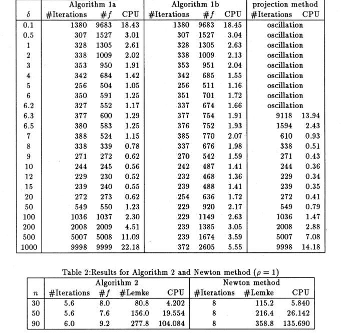
First we have compared Algorithms la, lb and the projection method (21) by using a 10-dimensional example, in which mapping $F$ is given by

The results for this problemare shown in Table 1.

In general, the projection method is guaranteed to converge, only if the parameter

6

is chosen sufficiently large. In fact, Table 1 shows that when

6

is large, the projection

methodis alwaysconvergent, but as $\delta$becomes small, thebehavior of the method becomes

unstable and eventually it fails to converge.

Table 1 also shows that Algorithms laand lb are always convergent even if

6

is chosen small, since line search determines an adequate step size at each iteration. Note that,

in Algorithm lb, the number of iterations is almost constant. This is because we may

choose a larger step size when the magnitude ofvector $d^{k}$ is small, i.e.

6

is large. This is

in contrast with Algorithm la, in which step size is bounded by 1 so that the number of iterations increases as $\delta$ becomes large.

Algorithms laand lb spendmore CPU times per iteration thanthe projection method,

because the formeralgorithmsrequireoverheads ofevaluatingthe merit function$f$

.

More-over, when $\delta$is between 0.1 and 20, Algorithm lb spends more CPU time than Algorithm

la, though the number of iterations are almost equal. This is because Algorithm lb

attempts to find a larger step size at each iteration. But, when

6

becomes large,

Algo-rithm lb tendsto spendless CPUtime thannotonlyAlgorithm labut alsothe projection

method, because the number of iterations ofAlgorithm lb does not increase so drastically.

4.2

Comparison of Algorithm 2 and Newton method

Next we have compared Algorithm 2 and the pure Newton method (18) without line

search. For each of the problem sizes $n=30,50$ and 90, we randomly generated five test problems. The parameters $\rho$ and

$\delta$ were set as

$\rho=1$ and $\delta=10$

.

The starting point was

chosen to be $x=0$

.

In solving the linearized subproblem at each iteration of Algorithm

2 and Newton method, we used Lemke’s complementarity pivoting method [10] coded

averages of the results for five problems for each case

_and#Lemke

is the total number of

pivotings in Lemke’s method.

Table 2 shows that the number of iterations of Newton method is consistently larger than that ofAlgorithm2 asfarasthetest problems usedintheexperiments are concerned. Therefore, since it is time consumingto solve alinear subproblem at each iteration,

Algo-rithm 2 required less CPU time than the pure Newton method in spite ofthe overheads

in line search. Finally we note that, the pure Newton method (18) is not guaranteed to

be globally convergent, although it actually converged for all test problems reported in

Table 2.

4.3

Comparison of

Algorithms

la

and

2

Finally we have compared Algorithms la and 2. For each of the problem sizes $n=$

$30,50$ and 90, we randomly generated five test problems. To see how these algorithms

behave for various degrees ofasymunetry ofthe mapping $F$, we have tested severalvalues of $\rho$ between 0.1 and 2.0. The starting point was chosen to be $x=0$

.

The results are

given in Table 3. All numbers shown in Table 3 are averages of the results for five test problems for each case.

Table 3 shows that when the mapping $F$ is close to symmetry, Algorithm la converges

very

fast, and when themapping becomes asymmetric, the number ofiterations and CPU time ofAlgorithm la increaserapidly. On the other hand, in Algorithm 2, while the total number of pivotings of Lemke’s method increases in proportion to problem size $n$, the

number ofiterations stays constant even when problem size and the degree of asymmetry

of $F$ are varied. Hence, when the degree of asymmetry of $F$ is relatively small, that is

when $\rho$ is smaller than 1.0, Algorithm la requires less CPU time than Algorithm 2.

Note that, since the mapping $F$ used in our computational experience is sparse, com-plexity of each iteration in Algorithm la is small. On the other hand, the code [8] of Lemke’s method used in Algorithm 2 to solve a hnear subproblem does not make use of sparsity, so that it requires a significant amount of CPU time at each iteration for large

problems. If a method that can make use of sparsity is available to solve a linear

sub-problem, CPU time of Algorithm 2 may decrease. The projected Gauss-Seidel method

[2, pp. 397] for solving linear complementarity problem is one of such methods. In Table

4, results of Algorithm 2 using the projected Gauss-Seidel method in place of Lemke’s

method are given. Table 4 shows that, if the mapping $F$ is almost symmetric, Algorithm

2 converges very fast. But Algorithm 2 fails to

converge

when the degree of

asymme-try increased, because the projected Gauss-Seidel method could not to find a solution to

linear subproblem.

with $n=30$ and 50. In

the

figure, the vertical axisrepresents the

accuracy

of a generated

point

to

the solution, which is evaluated by

ACC $= \max\{|\min(x_{i}, F_{1}(x))||i=1,2, \ldots, n\}$

.

(24)

Figure 1 indicates that Algorithm 2 is quadraticallyconvergent near the solution. Figure

1 also indicates that Algorithm la is linearly convergent though it has not been proved

theoretically.

$\ovalbox{\tt\small REJECT}\#X\Re$

[1] B. H. Ahn, “Solution ofNonsymmetric Linear Complementarity Problems by

Itera-tive Methods,” Journal

_of

optimization Theory and Applications 33 (1981) 175-185.

[2] R. W. Cottle, J. S. Pang and R. E. Stone, The Linear Complementarity Problem

(Academic Press, San Diego, 1992)

[3] S. Dafermos, (haffic _{Equilibrium and Variational Inequalities,” Transportation}

Sci-ence 14 (1980) 42-54.

[4] M. Florian, “Mathematical Programming Applications in National, Regional and

Urban Planning,” in: M. Iri and K. Tanabe eds., MathematicalProgramming: Recent Developments and Applications (KTKScientific Publishers, Tokyo, 1989) pp.283-307.

[5] M. Fukushima, “EquivalentDifferentiable optimization Problems and Descent Meth-odsfor AsymmetricVariationalInequality Problems,” Mathematical Programming53

(1992) 99-110.

[6] C. B. Garcia and W. I. Zangwill, Pathways to Solutions, FixedPoints, and Equilibria (Prentice-Hall, Eaglewood Cliffs N.J. 1981).

[7] P. T. Harker and J. S. Pang, (Finite-Dimensional _{Vaniational Inequality and}

Nonlin-ear Complementarity Problems: A Survey of Theory, Algorithms and Applications,”

Mathematical Programming 48 (1990) 161-220.

[8] T. Ibaraki and M. Fukushima, FORTRAN 77 optimization Programming (in

Japanese) (Iwanami-Shoten, Tokyo, 1991).

[9] N. H. Josephy, “Newton’s Method for Generalized Equations,” Technical Report No. 1965, Mathematics Research Center, University of Wisconsin (Madison, WI, 1979).

[10] C. E. Lemke, “Bimatrix Equilibrium Points and Mathematical Programming,” Man-agement Science 11 (1965) 681-689.

[11] O. L. Mangasarian and M. V. Solodov, “Nonlinear Complementarity as

Uncon-strained and ConUncon-strained Minimization,” Technical Report No. 1074, Computer

Sci-ences Department, University of$\cdot$Wisconsin (Madison, WI, 1992).

[12] L. Mathiesen, “An Algorithm based on a Sequence of Linear Complementarity

Prob-lems Applied to aWalrasian Equilibrium Model: An Example,” Mathematical

Pro-gramming 37 (1987) 1-18.

[13] J. S. Pang and D. Chan, “Iterative Methods for Variational and Complementarity Problems,” Mathematical Programming 24 (1982) 284-313.

[14] P. K. Subramanian, “Fixed Point Methods for The Complementarity Problem,”

Technical Report No. 2857, Mathematics Research Center, University of

Wiscon-sin (Madison, WI, 1985).

[15] K. Taji, M. Fukushima and T. Ibaraki, (A _{Globally Convergent Newton Method}

for Solving Strongly Monotone Variational Inequalities,” to appear in Mathematical

Programming.

[16] R. L. Tobin, (A _{Variable Dimension Solution Approach for the General Spatial Price}

Table l:Resultsfor Algorithm la, lb and the projection method $(n=10, \rho=1)$