Economics & Management Series EMS-2016-12
Education and Expenditure Inequality in Bhutan: An Analysis based on 2007 and 2012 Household Survey Data
Dorji Lethro
National Statistics Bureau, Royal Government of Bhutan
Takahiro Akita
Rikkyo University
October 2016
IUJ Research Institute
International University of Japan
These working papers are preliminary research documents published by the IUJ research institute. To facilitate prompt distribution, they have not been formally reviewed and edited. They are circulated in order to stimulate discussion and critical comment and may be revised. The views and interpretations expressed in these papers are those of the author(s). It is expected that the working papers will be published in some other form.
Education and Expenditure Inequality in Bhutan: An Analysis based on 2007 and 2012 Household Survey Data
Dorji Lethro
National Statistics Bureau, Royal Government of Bhutan e-mail: [email protected]
and Takahiro Akita
*Master of Public Management and Administration, Graduate School of Business, Rikkyo University
e-mail: [email protected] +81-90-2728-0272
ABSTRACT
Based on the 2007 and 2012 Bhutan Living Standard Survey, this study examines the roles of education in expenditure inequality in Bhutan using several decomposition techniques. While the expansion of basic education appears to have narrowed urban-rural expenditure disparity, the expansion of higher education seems to have increased expenditure inequality among households with higher education. Together with a rise in expenditure disparity among educational groups, this has raised overall expenditure inequality. Basic education policies that could raise general educational level still serve as an effective means to mitigate expenditure inequality.
Implementing effective higher education policies would be another important option, as the policies that could reduce inequality among households with higher education are crucial. There might be a mismatch between the needs of employers and the qualifications of people with higher education. The government thus needs to formulate and implement higher education policies that could mitigate the mismatch.
Keywords: education; expenditure inequality; decomposition of education Gini;
hierarchical decomposition of Theil index; Blinder-Oaxaca decomposition; Bhutan.
JEL: I24; I25; O15
Running Head: Education and Inequality in Bhutan
* The author is grateful to the Japan Society for the Promotion of Science for its financial support (Grant- in-Aid for Scientific Research 15K03473).
1 1. Introduction
Poverty and inequality are very important indicators of the living standard of people, and studies on these two topics are deemed important for developing countries like Bhutan. The National Statistics Bureau (NSB) has analyzed poverty every after conducting the Bhutan Living Standard Survey (BLSS), but it has not paid much attention to inequality. Analyses of inequality are very important as studies on poverty alone do not give overall picture of the living standard of people. Poverty indicators focus only on individuals or households who lie in the lower part of the distribution of expenditures or incomes, whereas inequality measures concern whole population.
The government of Bhutan implemented the first Five Year Plan (FYP) in 1961 in order to promote the socioeconomic development of the country. Prior to the first FYP, there were no motor roads for transportation and no electricity, and firewood was the only means of cooking and lighting houses. There were no communication services and people had to walk days and nights to take messages from one place to another. There were no proper education and health facilities, resulting in low literacy rate and life expectancy. People during that time period mainly depended on agriculture, livestock and forest for their livelihood. Since the first FYP was implemented, the government has been trying to improve the living standard of Bhutanese people through rural and social development. In the early 1980s, the gross enrollment rate (GER) of primary education was 57% and the GERs of secondary and tertiary education were, respectively, 11.2 and 0.7%. Over the last three decades, however, tremendous achievements have been made in education as the GERs of primary, secondary and tertiary education have increased respectively to 112, 92 and 37%
in 2015.
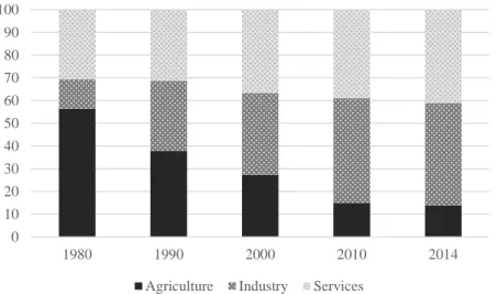
Real GDP has risen conspicuously over the last three decades. In 1980, it was merely Nu. 4,733 million, but increased to Nu. 12,101 million in 1990 and further increased to Nu.
54,835 million in 2014. Bhutan has also undergone massive changes in economic structure
(see Figure 1). Agriculture was the main source of income for the majority of people and the
GDP share of agriculture was 56% in 1980. However, its GDP share has declined
significantly over the last three decades, and in 2014, the agriculture sector accounts for only
14 %. On the other hand, the industry and service sectors grew rapidly and their GDP shares
have risen, respectively, to 45 and 41% from 14 and 30% between 1980 and 2014. Rapid
economic growth and concomitant changes in economic structure should have had massive
impacts on the distribution of incomes in Bhutan since people have been exposed to different
2
challenges and opportunities. Analyses of inequality are thus imperative for policy makers to formulate effective socio-economic development policies that are conducive to the reduction of inequality.
The main objective of this study is to explore the determinants of inequality in Bhutan based on household expenditure data from the 2007 and 2012 Bhutan Living Standard Survey (BLSS). This study focusses on education since education is found to be one of the major determinants of inequality. It analyzes the roles of education in expenditure inequality in an urban-rural dual framework using three decomposition methods: the decomposition of the educational Gini coefficient; the Blinder-Oaxaca decomposition; and the two-stage hierarchical decomposition of the Theil indices. By the decomposition of the educational Gini coefficient by location (urban and rural), we first examine educational inequality in an urban-rural dual framework. We next analyze the roles of education in urban-rural expenditure disparity by the Blinder-Oaxaca decomposition method. Finally, by using the two-stage hierarchical inequality decomposition method, we investigate the roles of education in expenditure inequality after eliminating the impact of urban-rural difference in educational endowments on expenditure inequality. To the best of our knowledge, this is the first study that explores the determinants of expenditure inequality in Bhutan using these three methods.
There have been a number of studies that have analyzed the effects of education on expenditure or income inequality.
1Among them, Tsakloglou (1993), Estudillo (1997), Akita, Lukman and Yamada (1999), Gray, Mills and Zandvakil. (2003), Mukhopadhaya (2003), Rao, Banerjee and Mukhopadhaya (2003) and Zaman and Akita (2012) employed a similar Theil decomposition method to explore possible determinants of income or expenditure inequality. According to them, education is one of the major determinants of income or expenditure inequality by accounting for around 20-40% of overall inequality. However, these studies used the one-stage inequality decomposition method, i.e., they conducted an inequality decomposition analysis according to some nominal scaled variables, such as age, education and gender, one at a time. Our study, on the other hand, employs the two-stage hierarchical inequality decomposition method, developed by Akita and Miyata (2013), to
1 See, for example, Knight and Sabot (1983), Ram (1989, 1990), Tsakloglou (1993), Park (1996), Estudillo (1997), Akita, Lukman and Yamada (1999), Chu (2000), De Gregorio and Lee (2002), Gray, Mills and Zandvakil. (2003),Mukhopadhaya (2003), Rao, Banerjee and Mukhopadhaya (2003), Borooah, Gustafsson, and Shi (2006), Lemieux (2006), Lin (2006), Liu (2006), Akita and Miyata (2008), Keller (2010), Földvária and van Leeuwenb (2011), Pieters (2011), Akita and Zaman (2012), Akita and Miyata (2013).
3
analyze the roles of education in an urban-rural dual framework. According to Akita and Miyata (2008), there is a large difference between the urban and rural sectors in the roles of education in inequality; while educational differences accounted for around 15% of urban inequality, they constituted merely 3-5% of rural inequality. This implies that inequality between educational groups is due in part to urban-rural differences in educational endowments. It is thus necessary to examine the roles of education in the urban and rural sectors separately.
2. Background Information on Bhutan
Bhutan is a small country, located on the southern slopes of eastern Himalayas and landlocked between China in the north and India in the east, west and south. The total territory measures approximately 38,394 square kilometers and more than 70% of the total land is covered by forest. According to the population projection of Bhutan
2, there were about 0.658 million people in 2007 and 0.720 million people in 2012. The current population is about 0.768 million. As an introduction to this study, regional structure, the structure of formal education and recent socioeconomic development are described briefly in this section.
2.1. Regional Structure
For administrative purposes, Bhutan is divided into 20 districts ( Dzongkhag ), each with a district officer (Dzongda), who is responsible for the well-being and developmental activities of the respective district (see Figure 2). Bigger districts (9 Dzongkhags) are divided further into one to three sub-districts (Dungkhag) and there are 16 Dungkhags in total. The lowest administrative unit called Gewog is formed by a group of Chiwogs . Gewog is administered by its council consisting of locally elected leader (Gup) and deputy ( Mangmi ) and Chiwog representatives (Tshogpa) .
There are at least one town in a Dzongkhag with defined boundaries, which are set by the Parliament upon recommendation of the Ministry of Works and Human Settlement.
These towns are usually referred to as urban areas, while the areas that fall within Gewogs are referred to as rural areas. However, for the survey purpose, some areas within Gewogs are considered as urban if most people in these areas are engaged in commercial activities and if most people earn income through non-agricultural activities.
2 National Statistical Bureau (NSB) has published the population projection of Bhutan 2005-2030 based on Population and Housing Census of Bhutan.
4 2.2. Structure of Formal Education
The modern education in Bhutan was started during the first king of Bhutan in 1914 by sending 46 students to India and also established two schools in the country. Until the late 1950s, monastic schooling was the predominant form of education. However, after the first five-year plan in 1961, modern education has been expanded. Now, Bhutan adopts seven- year primary education (Pre-primary – VI), followed by six-year secondary education (VII – XII) and then tertiary education (see Figure 3). Bhutan’s basic education is defined as eleven years of education, including primary plus four years of secondary education (Pre- primary – X). Government provides free education, and children begin their schooling at the age of six. After the completion of basic education, a certain proportion of students are enrolled in government higher secondary schools (XI – XII) based on the academic results.
The number of students enrolled depends upon the capacity of government higher secondary schools. The rest join private higher secondary schools, vocational training institutes or choose other opportunities. After completion of higher secondary school, most students are enrolled in undergraduate colleges in the country. But some are sent on scholarships outside the country based on the academic performance. The remaining students are enrolled in training institutes, which offer diploma courses within the country or find employment.
2.3. Recent Socioeconomic Development
The government started the First Five Year Plan (FYP) in 1961 in order to promote
the socioeconomic development, aiming towards the improvement of living standards of
Bhutanese people in the modern context. However, there was no adequate data to measure
the standard of living and welfare of the people quantitatively. Considering the importance
of information on living standard related indicators, the National Statistics Bureau (NSB)
conducted the First Bhutan Living Standard Survey (BLSS) in 2003. The objective of the
survey is to collect necessary information which could measure the standard of living and to
update the poverty profile of the country. Another objective is to assess the current FYP and
prepare socioeconomic policies for the next FYP. The First BLSS was conducted in the
beginning of the Ninth FYP (2002-2007) and the Second was conducted at the end of the
Ninth FYP in 2007. The information gathered in the First BLSS provided the baseline
information for the Ninth FYP, whereas the Second BLSS helped in assessing the
achievement of the plan. The latest survey (Third BLSS) was conducted in the fourth year
of the Tenth FYP (2008-2013), where the results were compared with the Second BLSS to
assess the achievement of the plan in improving the living standard of the people. Since this
5
study uses the Second and Third BLSS, we briefly describe the socioeconomic performance of the country during the Ninth and Tenth FYP as follows.
3The Ninth FYP was launched with the objective of improving the living standard and income of poor people, ensuring good governance, promoting the private sector for employment generation, preserving and promoting cultural heritage, conserving environment and achieving rapid economic growth. Over the plan period, real GDP grew at an annual average rate of 9.1% (see Figure 4), which exceeded the growth target of 8.2%.
Real GDP grew from Nu. 23.6 billion to 36.4 billion over the plan period. The main reason for this high growth was the sustained expansion of the electricity sector, which grew at an annual average rate of 29.4%. This rapid growth was achieved due mainly to tariff revisions for electricity exports and the generation of large income from the Tala Hydro-electric power project. However, the agriculture sector, which is the main income source for the majority of population, grew only at an annual average rate of 1.8%. The country experienced massive changes in the economic structure over the plan period, in which the GDP share of the agriculture sector declined from 25 to 18%, while the share of the industry sector increased from 40 to 46% and that of the service sector remained almost constant at 35%.
According to the Poverty Analysis Report (NSB, 2003), 31.7% of the people lived below the poverty line in 2003 (see Table 1). The poverty rate was much higher in rural areas than in urban areas (38.3% versus 4.2%). Due mainly to high economic growth, the national poverty rate declined notably to 23.2% in 2007 (NSB, 2007b). Rural and urban poverty rates also decreased to 30.9 and 1.7% respectively. Meanwhile, in 2003 overall inequality was very high at 0.416 as measured by the Gini index.
4However, it declined significantly to 0.352 in 2007. Rural and urban inequalities decreased also and were almost in the same level in 2007 at 0.32.
The Tenth FYP (2008-2013) was launched with the objective of poverty reduction through environmentally sustainable industrial development and integrated spatial and infrastructure development. Over the plan period, real GDP grew at an annual average rate of 6.7%; however, the country failed to achieve the growth target of 7.8%. Real GDP grew from Nu. 38.1 to 52.6 billion and per capita GDP rose from US$ 1,852.4 to US$ 2,440.4.
3 Gross National Happiness Commission of Bhutan (2003, 2009).
4 The officially published inequality as measured by the Gini index is different from this study. This is because the NSB used total consumption expenditure to compute the Gini coefficient, whereas this study uses per capita consumption expenditure.
6
The construction and wholesale and retail trade sectors grew rapidly at an annual average rate of 13.6 and 14.1%, respectively. The construction of three big hydropower projects ( Punatsangchu I and II and Mangdechhu ) during the Tenth FYP has contributed a lot to the rapid growth of the construction sector. Like the Ninth FYP, the agriculture sector experienced the slowest growth at 2.2%; thus the GDP share of the agriculture sector declined from 17 to 14 %. The share of the industry sector also declined, but very slightly from 47 to 46%. Meanwhile, the share of the service sector increased from 36 to 40%.
The government attempted to bring down the poverty rate to 15% during the Tenth FYP. According to the 2012 Poverty Analysis Report (NSB, 2012b), however, the poverty rate actually declined to 12% in 2012. While the incidence of poverty remained almost constant in urban areas at 1.8%, it declined substantially to 16.7% in rural areas. On the other hand, overall inequality increased to 0.360 in 2012. Both urban and rural inequalities rose also to 0.350 and 0.340, respectively.
3. Data and Methods
3.1. Data: Bhutan Living Standard Survey (BLSS)
The National Statistics Bureau (NSB) has been conducting the Bhutan Living Standard Survey (BLSS) based on the methodology of World Bank’s Living Standard Measurement Study (LSMS). The latest survey was conducted in 2012. It is a nation-wide survey to study the living standard of Bhutanese people and collected information on demography, education, health and employment of each household member. The survey also collected information on housing condition, asset, income, and consumption expenditure of households. This study uses expenditure data from the 2007 and 2012 BLSS to perform an inequality decomposition analysis by location (urban and rural) and educational attainment of household head.
5The number of households surveyed in the 2007 BLSS is 9,798, of which 2,942 and 6,856 households are, respectively, in the urban and rural sectors. On the other hand, 8,968 households are sampled in the 2012 BLSS, of which 4,619 and 4,349 are, respectively, in the urban and rural sectors. In the survey, monthly household consumption expenditures are collected for both food and non-food items. Since the prices of these items differ across regions, the Paasche index is used as a regional deflator to convert nominal expenditures to real expenditures.
5 National Statistical Bureau (2007a, 2012a).
7
In inequality decomposition analyses, households are classified into four education groups (no education, primary, secondary and tertiary) depending upon the highest grade the household head had completed (see Figure 3). No education group includes those households whose heads had never attended formal education. Primary education group includes those households whose heads had attended pre-primary education or grade 1-6. Secondary education group includes those households whose heads had attended grade 7-12 or vocational training institutes. Finally, tertiary education group includes those households whose heads had attended diploma courses or above.
Using sampling weights, the distribution of households across the four educational groups is estimated in the urban and rural sectors, as shown in Table 2. The majority of household heads do not have formal education and most of them are residing in rural areas.
However, the expansion of education seems to have occurred gradually between 2007 and 2012, as the proportion of households with no education has declined from 68 to 60%, while the proportion of households with secondary and tertiary education has risen from 18 to 26%.
Table 2 also presents the urban-rural distribution of households. Urbanization appears to have proceeded steadily as the urban sector’s share of households has risen from 30 to 34%.
One possible factor of the rise in the urban share would be the increase in the number of high school and college graduates who have entered urban labor markets and started living independently in urban areas. It should be noted that the share of households with secondary and tertiary education has risen significantly from 45% to 53% in the urban sector.
3.2. Methods
3.2.1. Decomposition of Educational Gini Coefficient by Urban and Rural Locations
In order to examine the determinants of educational inequality, we conduct an
inequality decomposition analysis by location (urban and rural sectors) using the Gini
coefficient. The Gini coefficient satisfies several desirable properties as a measure of
inequality, such as anonymity principle, income homogeneity, population homogeneity and
the Pigue-Dalton principle of transfer (Anand 1983). Unlike the generalized entropy class of
inequality measures including the Theil indices, however, we cannot decompose total
inequality additively into the within and between-sector components. This is because an
additional term emerges if there is an overlap between the urban and rural sectors in the
distribution of educational attainments. Nonetheless, we use the Gini coefficient to analyze
educational inequality in an urban and rural framework since it is interesting to know the
8
magnitude of overlap in the distribution of educational attainments between the urban and rural sectors.
6Let us assume that there are N households in an economy, which are categorized into the urban and rural sectors and the number of years of education completed by the household head represents the educational level of the household. Then, overall educational inequality, as measured by the Gini coefficient, is given by:
(1) where 𝑒𝑒
𝑖𝑖ℎand 𝑒𝑒
𝑗𝑗𝑗𝑗= number of years of education of household ℎ in sector 𝑖𝑖 and household
𝑘𝑘 in sector 𝑗𝑗 respectively ,
𝜇𝜇 = mean years of education of all households, and
𝑁𝑁
𝑖𝑖and 𝑁𝑁
𝑗𝑗= total number of households in sector 𝑖𝑖 and 𝑗𝑗 respectively.
As mentioned above, this education Gini is decomposed additively into the within-sector ( G
WS)
,between-sector ( G
BS) and residual ( G
R) components as follows (Lambert and Aronson 1993; Dagum 1997).
R BS
WS
G G
G
G = + + (2)
In this equation, G
WSis the weighted average of the urban and rural Gini coefficients and given by:
= ∑
= 2 i 1 i i i
WS
p s G
G (3) where p
i= share of sector i in the total number of households ,
s
i= share of sector 𝑖𝑖 in the total number of years of education, and G
i= education Gini of sector 𝑖𝑖.
On the other hand, G
BSis the education Gini that is obtained when each household in a sector is assigned the mean number of years of education for the sector and defined by:
∑∑
∑∑∑∑
= = = = = =−
=
−
=
21 2
1 2
1 2
1 1 1
2
2
1 2
1
i j i j i j
i j
N h
N
k i j
BS
p p μ μ
μ μ μ μ
G N
i j(4)
where μ
iand μ
j= mean years of education in sector 𝑖𝑖 and 𝑗𝑗 respectively.
6 We should note that since household heads who have no education have 0 year of education, it is not possible to calculate the Theil indices.
9
Lastly, the residual term, G
R= G − G
WS− G
BS, will take a positive value if the educational distributions for the urban and rural sectors overlap, while it will be zero if they do not overlap.
3.2.2. Blinder-Oaxaca Decomposition
To examine the extent to which the difference in educational endowments between the urban and rural sectors explain the urban-rural expenditure disparity, we employ the Blinder- Oaxaca decomposition method (Blinder 1973; Oaxaca 1973). We consider the following linear regression model for per capita household expenditure in the urban and rural sectors:
k k k
k
e
y = X ' β + E ( e
k) = 0 k = U , R where y
k= natural log of per capita expenditure,
X
k= a vector of explanatory variables,
β
k= a vector of coefficients associated with explanatory variables and e
k= error term.
Then the estimated urban-rural difference in mean per capita expenditure can be decomposed additively into the following two components (Neumark 1988).
( ' ( ˆ ˆ *) ' ( ˆ * ˆ ) )
ˆ * )' ˆ (
R R
U U R
U R
U
y
y
D = − = X − X β + X β − β + X β − β (5)
where β ˆ = a vector of the least square estimates which are obtained individually from the
kurban and rural samples,
ˆ *
β = a vector of the least square estimates which are obtained from the pooled sample of urban and rural households, and
X
k= estimate of E ( X
k) .
The first component in equation (5) presents the urban-rural expenditure difference due to explanatory variables (endowment effect), whereas the second component denotes the unexplained part. Explanatory variables included in the regression model are years of education, age, age squared, gender, marital status and household size.
3.2.3. Hierarchical Decomposition of Inequality by the Theil index T
We perform a hierarchical decomposition analysis of expenditure inequality by
location and education using the Theil index T to examine the roles of education in
10
expenditure inequality in an urban-rural dual setting.
7Like the Gini coefficient, the Theil index T satisfies anonymity principle, income homogeneity, population homogeneity and the Pigue-Dalton principle of transfer (Anand 1983). Furthermore, it is additively decomposable, i.e., overall inequality, as measured by the Theil index T , can be decomposed additively into the within- and between-group components (Bourguignon 1979; Shorrocks 1980).
Based on the hierarchical Theil decomposition method proposed by Akita and Miyata (2013), all households are first grouped into the urban and rural sectors and households in each of these two sector are classified further into four educational groups: no education, primary, secondary and tertiary education groups. Then overall expenditure inequality as measured by the Theil index T is given by:
= ∑∑∑
= = =
N
y Y Y
T y
ijk
i j
N k
ij ijk
log 1
2
1 4
1 1
(6)
where y
ijk= household k’s per capita expenditure in educational group 𝑗𝑗 in sector 𝑖𝑖 , Y = total per capita expenditure of all households, and
N
ij= total number of households in educational group 𝑗𝑗 in sector 𝑖𝑖.
According to Akita and Miyata (2013), equation (6) can be decomposed hierarchically into the between-sector ( T
BS), within-sector between-group ( T
WSBG) and within-sector within-group inequality components ( T
WSBG) as follows:
∑ ∑
+
∑
+
=
= = =2 1
4 1 2
1 i j ij ij
i BGi
BS i
T
Y T Y
Y T Y
T = T
BS+ T
WSBG+ T
WSWG. (7)
where T
BS= inequality between the urban and rural sectors, T
BGi= inequality between educational groups in sector 𝑖𝑖 T
ij= inequality within educational group 𝑗𝑗 in sector 𝑖𝑖,
Y
i= total per capita expenditure of households in sector i , and
Y
ij= total per capita expenditure of households in educational group j in sector i.
7 The Theil index L is also used to conduct a hierarchical inequality decomposition analysis. But the result is very similar to the one by the Theil index T qualitatively; thus the result based on the Theil index T is only presented in this paper.
11
We can reverse the order of decomposition in the hierarchical decomposition method, i.e., all households are first classified into four education groups and then households in each educational group are classified into the urban and rural sectors. We can thus decompose overall expenditure inequality hierarchically into the between-group ( T
BG), within-group between-sector ( T
WGBS) and within-group within-sector ( T
WGWS) inequality components as follows;
WGWS WGBS
BG
T T
T
T = + + (8) It should be noted that T
WSWGobtained in equation (7) and T
WGWSobtained in equation (8) are the same since we have
j i ij WGWS
ij
i j ij
ij
WSWG
T T
Y T Y
Y
T Y =
=
= ∑∑ ∑∑
= =
= =
4
1 2
1 2
1 4
1
Therefore, the order of decomposition matters in the hierarchical decomposition method. Tang and Petrie (2009) suggested an alternative multivariate decomposition method called the non-hierarchical decomposition method in order to rectify this problem. In the non-hierarchical decomposition method, overall inequality is decomposed simultaneously with respect to some nominal scaled variables such as education, location, gender, ethnicity and age. In the location and education context, overall inequality is decomposed non- hierarchically as follows:
WSWG ISG
BG
BS
T T T
T
T = + + + (9) where T
ISG= interaction term between location and education.
From equations (7) and (9), the interaction term is given by T
ISG= T
WSBG− T
BG, which can be positive or negative. Though the interaction term indicates that there are urban-rural differences in the role of education in expenditure inequality, the non-hierarchical decomposition technique fails to analyze the role of education in expenditure inequality in each of the urban and rural sectors.
4. Empirical Results
4.1. Mean per capita Expenditure and Mean Years of Education in the Urban and Rural Sectors
Table 3 presents mean per capita expenditure for four educational groups in the urban
and rural sectors. The urban-rural disparity in mean per capita expenditure was 2.2 in 2007,
but has declined notably to 1.8 in 2012. In 2007, no education group had the largest urban-
12
rural disparity at 2.1, which was followed by primary, secondary and tertiary education groups. In 2012, all but tertiary group reduced their urban-rural expenditure disparity. No education group had still the largest urban-rural disparity at 1.5 in 2012, but much smaller than the disparity in 2007. An interesting fact is that tertiary education group raised its urban- rural disparity, and in 2012, the disparity increased to 1.4, which is in fact larger than the ones registered by primary and secondary education groups. This indicates that labor demands for college graduates have expanded rapidly in the urban sector.
Education is considered to be one of the major determinants of wage income, and a positive relationship is thought to exist between the distribution of income and educational inequality. Whether educational expansion has widened or narrowed educational inequality is thus of policy relevance. Table 3 also exhibits mean number of years of education for the urban and rural sectors. Mean number of years of education was 2.9 in 2007 in Bhutan as a whole, but has risen conspicuously to 3.9 in 2012. The expansion of education was faster in the rural than in the urban sector in the period. While mean number of years of education has increased from 6.6 to 7.5 in the urban sector, it has risen from 1.3 to 2.1 in the rural sector; thus, the urban-rural ratio in mean number of years of education has declined substantially from 5.1 to 3.6 though it is still very high by international standards. The expansion of education in this period has therefore narrowed the educational disparity between the urban and rural sectors. Next question is whether this educational expansion has widened or narrowed educational inequality within the urban and rural sectors and overall educational inequality. In order to answer the question, we conduct a decomposition analysis of educational inequality by urban and rural sectors using the Gini coefficient.
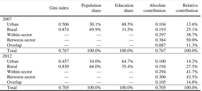
4.2. Decomposition of Educational Gini Coefficient by Urban and Rural Sectors
Table 4 presents the result of the decomposition of educational Gini coefficient by
urban and rural sectors. Overall educational inequality was 0.77 in 2007 as measured by the
Gini coefficient, but with the expansion of secondary and tertiary education it has declined
slightly to 0.71 in 2012. Educational inequality is much smaller in the urban than the rural
sector. It has declined in both the urban and rural sectors between 2007 and 2012: from 0.51
to 0.46 in the urban sector and from 0.87 to 0.83 in the rural sector. Educational inequality
within the urban sector accounted for 14% of overall educational inequality in 2007, and its
contribution has remained almost constant in 2012. Meanwhile, rural sector’s educational
inequality constituted 25% of overall educational inequality in 2007, but its contribution has
risen to 28% in 2012.
13
The expansion of secondary and tertiary education appears to have lowered not only educational inequality within the urban and rural sectors but also educational disparity between these two sectors, as the between-sector Gini coefficient has declined significantly from 0.38 to 0.31 and its contribution to overall educational inequality has decreased from 50 to 44%. The decrease in the between-sector Gini coefficient seems to have been the main contributor to the fall in overall educational inequality. Meanwhile, the contribution of the residual term, which represents the overlap in the distribution of educational attainment between the urban and rural sectors, has risen notably from 11 to 15%.
In order to analyze the extent to which the urban-rural expenditure disparity is explained by the urban-rural difference in the level of educational attainments, we next conduct a Blinder-Oaxaca decomposition analysis.
4.3 Blinder-Oaxaca Decomposition of the Urban-Rural Difference in Mean per capita Expenditure
Table 6 presents the result of a Blinder-Oaxaca decomposition analysis, while Table 5 shows summary information on the variables used in the decomposition analysis. The urban- rural difference in educational endowments seems to have played an important role in determining the expenditure disparity between the urban and rural sectors, as the urban-rural difference in mean number of years of education accounts for 25% of the urban-rural expenditure difference in 2007 and its contribution increased substantially to 40% in 2012.
According to Table 2, 76% of rural households do not have formal education in 2012, which is compared to 31% of urban households. It is thus imperative to promote basic education and raise the general level of education in the rural sector to narrow the urban-rural expenditure gap.
The decomposition result suggests however that there are many other factors that could
account for the expenditure difference between the urban and rural sectors, as the
unexplained part contributes more than 50% of the expenditure difference: 68% in 2007 and
54% in 2012. Among them would be the difference in job types between the urban and rural
sector. While most of rural households are engaged in agricultural activities, urban
households are engaged in a variety of economic activities, mainly in the industrial and
services sectors. This should have exerted substantial effects on the urban-rural difference
in wage income and thus consumption expenditure.
14
4.4 Hierarchical Decomposition of Expenditure Inequality by Location (Urban and Rural) and Education by the Theil index T
We now conduct a hierarchical inequality decomposition analysis by location (urban and rural) and education using the Theil index T in order to analyze the roles of education in expenditure inequality in an urban-rural dual setting. Table 7 presents the result.
8Overall expenditure inequality, as measured by the Theil index T , has increased from 0.287 to 0.330 between 2007 and 2012. Rural expenditure inequality has risen from 0.220 to 0.276 and its contribution to overall inequality has increased slightly from 40 to 43%. But the main contributor to the rise in overall expenditure inequality appears to have been the increase in urban inequality. Between 2007 and 2012, urban inequality has risen significantly from 0.208 to 0.301, and its contribution to overall inequality has increased prominently from 35 to 44%. Unlike many other countries, in 2007 urban inequality was smaller than rural inequality (0.208 against 0.220), but the former became larger than the latter in 2012 (0.301 against 0.276).
9This may be a consequence of rural-to-urban migration of households with higher education. As shown in Table 3, in 2007 the urban sector has a much larger mean per capita expenditure than the rural sector; the urban-rural ratio was 2.2. Thus there was a large incentive for those rural households with higher education to migrate to the urban sector which offers a variety of job opportunities.
At the same time, the expansion of basic education has taken place in the rural sector.
As a consequence, the urban-rural disparity in educational attainment has narrowed (see Table 3), resulting in the decline in the urban-rural expenditure disparity (i.e., between-sector inequality) between 2007 and 2012 as shown by Table 7. The contribution of the urban-rural disparity to overall inequality has declined prominently from 25 to 13%. In contrast, that of the within-sector inequality component (i.e., a weighted average of urban and rural inequalities) has risen substantially from 75 to 87%. As discussed above, however, most of the increase is attributable to the rise in urban expenditure inequality.
As shown by the Blinder-Oaxaca decomposition, education was one of the major contributors to the urban-rural expenditure disparity. The question arises as to the roles of education in expenditure inequality within the urban and rural sectors. We now perform a decomposition analysis of expenditure inequality by educational groups. According to Table
8 Table A1 in the Appendix provides the results of one-stage inequality decomposition by urban and rural locations and one-stage decomposition by education in each of the urban and rural sectors. The result of a two- stage hierarchical decomposition analysis summarizes these results.
9 See, for example, Eastwood and Lipton (2004), Shorrocks and Wan (2005) and Kanbur and Zhuang (2013).
15
8, which exhibits the result of a non-hierarchical inequality decomposition analysis together with that of a hierarchical inequality decomposition analysis, there is a large negative interaction effect. This implies that expenditure inequality among four educational groups is due in part to the difference in the level of educational attainment between the urban and rural sectors. It is imperative, therefore, to analyze the roles of education in the urban and rural sectors separately.
Table A1 in the Appendix exhibits the result of a one-stage inequality decomposition analysis by educational groups in each of the urban and rural sectors, which is incorporated in Table 7 in the framework of a hierarchical inequality decomposition analysis by location (urban and rural) and education. As presented above, urban inequality has risen significantly between 2007 and 2012 and its contribution to overall inequality has risen from 35 to 44%.
All but no education group registered an increase in expenditure inequality in the urban sector. Particularly, the secondary and tertiary education groups raised their inequalities significantly and their combined contribution to overall expenditure inequality has gone up from 16 to 28%. At the same time, inequality between four educational groups has increased from 0.020 to 0.044 and its contribution has risen from 3 to 6%. These observations suggest that the expansion of higher education in the urban sector has accompanied by a rapid rise in expenditure inequality within secondary and tertiary education groups as well as between four education groups.
Rural inequality has increased also, but to a lesser extent and its contribution to overall inequality has risen from 40 to 43%. All but tertiary education group has experienced an increase in expenditure inequality. But the major contributor to the increase in rural inequality appears to have been the secondary education group, which raised its expenditure inequality from 0.188 to 0.240. It should be noted that tertiary education group has lowered its expenditure inequality, but its contribution to overall inequality has increased due to a substantial rise in expenditure share.
In sum, while the contribution of the between-sector component (BS) has declined
from 25 to 13% between 2007 and 2012, those of the within-sector between-group
component (WSBG) and the within-sector within-group component (WSWG) have risen,
respectively, from 8 to 12% and from 66 to 75% (see Table 7).
16 5. Conclusions
Based on the 2007 and 2012 Bhutan Living Standard Survey (BLSS), this study analyzed the roles of education in expenditure inequality in Bhutan using several decomposition techniques. The major findings are summarized as follows. Around 60% of household heads do not have formal education and most of them live in the rural areas. But, with the expansion of basic education, particularly in the rural sector, the educational disparity between the urban and rural sectors has decreased notably as the urban-rural ratio in mean number of years of education has declined from 5.1 to 3.6. At the same time, the urban-rural overlap in the distribution of educational attainments has risen. Overall educational inequality, as measured by the Gini coefficient, has fallen from 0.77 to 0.71 between 2007 and 2012, but this is due mainly to a decrease in the urban-rural educational disparity.
According to a Blinder-Oaxaca decomposition analysis, the urban-rural difference in educational endowments seems to have been one of the key determinants of the urban-rural expenditure disparity, which is still very high, particularly among households with lower education. While the expansion of basic education, particularly in the rural sector, appears to have narrowed the expenditure disparity between the urban and rural sectors, the expansion of higher education seems to have increased expenditure inequality among households with higher education, particularly in the urban sector. Together with a rise in expenditure disparity among educational groups, particularly between higher and lower educational groups in the urban sector, this has raised overall expenditure inequality between 2007 and 2012.
Some policy implications can be drawn from these findings. Basic education policies
that could raise general educational level, particularly in rural areas, still serve as an effective
means to mitigate expenditure inequality in Bhutan. By these policies, we could reduce the
educational disparity between the urban and rural sectors and thus mitigate the expenditure
disparity between them, as education appears to have been one of the key determinants of
the urban-rural expenditure disparity. Implementing effective higher education policies,
particularly in the urban sector, would be another important policy option. Since the
expansion of higher education seems to have been one of the key determinants of a rise in
overall expenditure inequality, higher education policies that could reduce expenditure
inequality among households with higher education are crucial. There might be a mismatch
between the needs of employers and the qualifications of people with higher education in
17
the labor market. To reduce expenditure inequality, therefore, the government needs to formulate and implement effective higher education policies that could mitigate the mismatch in the labor market. Given the paucity of higher education institutions, vocational training programs could play a key role in Bhutan.
References
Akita, Takahiro; Rizal Affandi Lukman, and Yukino Yamada. 1999. “Inequality in the Distribution of Household Expenditures in Indonesia: A Theil Decomposition Analysis.” The Developing Economies 37, no. 2: 197-221.
Akita, Takahiro, and Sachiko Miyata. 2008. “Urbanization, Educational Expansion, and Expenditure Inequality in Indonesia in 1996, 1999, and 2002.” Journal of the Asia Pacific Economy 13, no. 2: 147-167.
Akita, Takahiro, and Sachiko Miyata. 2013. “The Roles of Location and Education in the Distribution of Economic Well-being in Indonesia: Hierarchical and Non- hierarchical Inequality Decomposition Analyses.” Letters in Spatial and Resource Sciences 6, no. 3: 137-150.
Anand, Sudhir. 1983. Inequality and Poverty in Malaysia: Measurement and Decomposition . New York: Oxford University Press.
Blinder, Alan S. 1973. “Wage Discrimination: Reduced Form and Structural Estimates.”
Journal of Human Resources 8, no. 4: 436–55.
Bourguignon, Francois. 1979. “Decomposable Income Inequality Measures.” Econometrica 47, no. 4: 901-920.
Commission for Development Research. 2010. The Education System in Bhutan & Austro- Bhutanese Development and Research Co-operation.
Chu, Hong-Yih. 2000. “The Impacts of Educational Expansion and Schooling Inequality on Income Distribution.” Quarterly Journal of Business and Economics 39, no. 2: 39- 49.
Dagum, Camilo. 1997. “A New Approach to the Decomposition of the Gini Income Inequality Ratio.” Empirical Economics 22: 515-531.
Gray, David; Jeffrey A. Mills; and Sourushe Zandvakili. 2003. “Statistical Analysis of Inequality with Decompositions: the Canadian Experience.” Empirical Economics 28: 291-302.
De Gregorio, Jose and Jong-Wha Lee. 2002. “Education and Income Inequality: New Evidence from Cross-country Data.” Review of Income and Wealth 48, no. 3: 395- 416.
Eastwood, Robert, and Michael Lipton. 2004. “Rural and Urban Income Inequality and
Poverty: Does Convergence between Sectors Offset Divergence within Them?” In
Inequality, Growth, and Poverty in an Era of Liberalization and Globalization ,
edited by G. A. Cornia. Oxford: Oxford University Press.
18
Estudillo, Jonna P. 1997. “Income Inequality in the Philippines, 1961–91.” The Developing Economies 35, no. 1: 68–95.
Foldvaria, Peter, and Bas van Leeuwenb. 2011. “Should Less Inequality in Education Lead to a More Equal Income Distribution?” Education Economics 19, no. 5: December 2011, 537–554
Gross National Happiness Commission of Bhutan. 2003. Ninth Five Year Plan, Volume I and II. Thimphu: Royal Government of Bhutan.
Gross National Happiness Commission of Bhutan. 2009. Tenth Five Year Plan, Volume I and II. Thimphu: Royal Government of Bhutan.
Kanbur, Ravi, and Juzhong Zhuang. 2013. “Urbanization and Inequality in Asia.” Asian Development Review 30, no. 1: 131–147.
Keller, Katarina R.I. 2010. “How Can Education Policy Improve Income Distribution?: An Empirical Analysis of Education Stages and Measures on Income Inequality.” The Journal of Developing Areas 43, no. 2: 51-77.
Knight, John B., and Richard H. Sabot. 1983. “Educational Expansion and the Kuznets Effect.” The American Economic Review 73, no. 5: 1132-1136.
Lambert, Peter J., and J. Richard Aronson. 1993. “Inequality Decomposition Analysis and the Gini Coefficient Revisited.” The Economic Journal 103: 1221-1227.
Lemieux, Thomas. 2006. “Postsecondary Education and Increasing Wage Inequality.” The American Economic Review 96, no. 2: 195-199
Lin, Chun-Hung A. 2006. “Educational Expansion, Educational Inequality, and Income Inequality: Evidence from Taiwan, 1976-2003.” Social Indicators Research 80: 601- 615.
Liu, Amy Y. C. 2006. “Changing Wage Structure and Education in Vietnam, 1992–98: The Roles of Demand.” Economics of Transition Volume 14, no. 4: 681–706
Mukhopadhaya, Pundarik. 2003. “Trends in Total and Subgroup Income Inequality in the Singaporean Workforce.” Asian Economic Journal 17, no. 3: 243-264.
National Statistics Bureau (NSB). 2003. Poverty Analysis Report 2003 . Thimphu: Royal Government of Bhutan.
National Statistics Bureau (NSB). 2007a. Second Bhutan Living Standard Survey (BLSS) . Thimphu: Royal Government of Bhutan.
National Statistics Bureau (NSB). 2007b. Poverty Analysis Report 2007 . Thimphu: Royal Government of Bhutan.
National Statistics Bureau (NSB). 2012a. Third Bhutan Living Standard Survey (BLSS) , Thimphu: Royal Government of Bhutan.
National Statistics Bureau (NSB). 2012b. Poverty Analysis Report 2012 . Thimphu: Royal Government of Bhutan.
National Statistics Bureau (NSB). 2002-2014. National Accounts Statistics . Thimphu: Royal Government of Bhutan.
Neumark, David. 1988. “Employers’ Discriminatory Behavior and the Estimation of Wage
Discrimination.” Journal of Human Resources 23, no.3: 279–95.
19
Oaxaca, Ronald. 1973. “Male–female Wage Differentials in Urban Labor Markets.”
International Economic Review 14, no. 3: 693–709.
Park, Kang H. 1996. “Educational Expansion and Educational Inequality on Income Distribution.” Economics of Education Review 15, no. 1: 51-58.
Pieters, Janneke. 2011. “Education and Household Inequality Change: A Decomposition Analysis for India.” The Journal of Development Studies 47, no. 12: 1909-1924.
Ram, Rati. 1989. “Can Educational Expansion Reduce Income Inequality in Less-Developed Countries?” Economics of Education Review 8, no. 2: 185-195
Ram, Rati. 1990. “Educational Expansion and Schooling Inequality: International Evidence and Some Implications.” The Review of Economics and Statistics 72, no. 2: 266-274.
Rao, V. V. Bhanoji; D.S. Banerjeel; and Punkarik Mukhopadhaya. 2003. “Earnings Inequality in Singapore.” Journal of the Asia Pacific Economy 8, no. 2: 210-228.
Shorrocks, Anthony. 1980. “The Class of Additively Decomposable Inequality Measures.”
Econometrica 48, no. 3: 613–25.
Shorrocks, Anthony, and Guanghua Wan. 2005. “Spatial Decomposition of Inequality.”
Journal of Economic Geography 5, no. 1: 59-81.
Tang, Kim Ki, and Dennis Petrie. 2009. “Non-hierarchical Bivariate Decomposition of Theil Indexes.” Economics Bulletin 29, no. 2: 928-927.
Tsakloglou, Panos. 1993. “Aspects of Inequality in Greece: Measurement, Decomposition and Intertemporal Change, 1974, 1982.” Journal of Development Economics 40, no.
1: 53–74.
Zaman, K. A. Uz and Takahiro Akita. 2012. “Spatial Dimensions of Income Inequality and
Poverty in Bangladesh: An Analysis of the 2005 and 2010 Household Income and
Expenditure Survey Data.” Bangladesh Development Studies 35, no. 3: 19-51.
20
Table 1: Poverty and Inequality
Area 2003 2007 2012
Poverty rate Inequality Poverty rate Inequality Poverty rate Inequality
Urban 4.2 0.374 1.7 0.317 1.8 0.350
Rural 38.3 0.381 30.9 0.315 16.7 0.340
National 31.7 0.416 23.2 0.352 12 0.360
Source: Poverty Analysis Report (2003, 2007, 2012), NSB
Table 2: Distribution of Households across Educational Groups in the Urban and Rural Sectors
Household distribution across educational group in each sector (%)
Urban and rural shares (%) No education Primary Secondary Tertiary
2007
Urban 35.2 19.4 34.7 10.6 30.1
Rural 81.8 11.3 5.8 1.1 69.9
Total 67.8 13.7 14.5 4.0 100.0
2012
Urban 30.5 16.7 37.7 15.1 34.0
Rural 75.6 11.7 9.0 3.6 66.0
Total 60.3 13.4 18.8 7.5 100.0
Table 3: Mean per capita Expenditure and Mean Number of Years of Education in the Urban and Rural Sectors
Mean per capita expenditure in Ngultrum (Nu) Mean years of education No education Primary Secondary Tertiary Total
2007
Urban 3,906 3,604 4,872 6,726 4,482 6.59
Rural 1,890 2,155 3,646 5,640 2,064 1.31
Total 2,206 2,771 4,529 6,514 2,748 2.90
U-R ratio 2.07 1.67 1.34 1.19 2.17 5.05
2012
Urban 5,628 5,748 8,513 12,451 7,765 7.47
Rural 3,763 4,418 6,959 9,048 4,321 2.10
Total 4,084 4,983 8,019 11,365 5,493 3.93
U-R ratio 1.50 1.30 1.22 1.38 1.80 3.55
21
Table 4: Decomposition of Educational Gini Coefficient by Location (Urban and Rural)
Gini index Population
share
Education share
Absolute contribution
Relative contribution 2007
Urban 0.506 30.1% 68.5% 0.104 13.6%
Rural 0.874 69.9% 31.5% 0.193 25.1%
Within-sector --- --- --- 0.297 38.7%
Between-sector --- --- --- 0.384 50.0%
Overlap --- --- --- 0.087 11.3%
Total 0.767 100.0% 100.0% 0.767 100.0%
2012
Urban 0.457 34.0% 64.7% 0.100 14.2%
Rural 0.830 66.0% 35.4% 0.194 27.5%
Within-sector --- --- --- 0.294 41.7%
Between-sector --- --- --- 0.306 43.5%
Overlap --- --- --- 0.105 14.8%
Total 0.705 100.0% 100.0% 0.705 100.0%
Table 5: Summary Statistics
Variable Urban Rural
Obs. Mean Std. Dev. Min Max Obs. Mean Std. Dev. Min Max 2007
Household size 2,942 4.40 1.94 1 15 6,856 5.28 2.41 1 19
Age 2,942 37 11.33 17 93 6,856 49 14.58 14 102
Gender 2,942 0.79 0.41 0 1 6,856 0.65 0.48 0 1
Marital status 2,942 0.85 0.35 0 1 6,856 0.78 0.41 0 1
Per capita exp. 2,942 4,482 3,439 477 74,659 6,856 2,064 1,607 228 24,678
Years of education 2,942 6.59 5.98 0 22 6,856 1.31 3.25 0 22
2012
Household size 4,619 4.14 1.71 1 16 4,349 4.75 2.21 1 17
Age 4,619 39 12.12 15 103 4,349 49 15.34 17 102
Gender 4,619 0.81 0.40 0 1 4,349 0.66 0.48 0 1
Marital status 4,619 0.83 0.37 0 1 4,349 0.80 0.40 0 1
Per capita exp. 4,619 7,765 8,056 717 182,456 4,349 4,321 4,328 165 96,032
Years of education 4,619 7.47 6.07 0 22 4,349 2.10 4.35 0 22
22
Table 6: Blinder-Oaxaca Decomposition of the Urban-Rural Differences in Mean per capita Expenditure
2007 2012
Coefficient Z-value % Contr. Coefficient Z-value % Contr.
Differential
Prediction for urban 8.208 778.74 8.711 905.36
Prediction for rural 7.430 1033.67 8.131 841.25
Difference 0.779 61.03 100.0 0.580 42.53 100.0
Explained
Years of Education 0.198 24.69 25.4 0.230 29.03 39.6
Age -0.252 -10.14 -32.3 -0.138 -5.61 -23.8
Age squared 0.228 9.73 29.3 0.123 5.21 21.1
Household size 0.101 17.85 12.9 0.073 13.36 12.7
Gender -0.020 -9.44 -2.6 -0.018 -7.76 -3.2
Marital status -0.004 -3.17 -0.5 -0.002 -2.81 -0.4
Total 0.251 24.99 32.3 0.267 26.36 46.0
Unexplained
Total 0.527 32.4 67.7 0.313 23.96 54.0
Table 7: Two-stage Hierarchical Decomposition of the Theil index T for all Households
Components
Theil Index T Expenditure Share (%)
2007 2012
2007 2012
Inequality % Contr. Inequality % Contr.
Total 0.287 100.0 0.330 100.0 100.0 100.0
B-Sector (BS) 0.073 25.4 0.042 12.7
W-Sector B-Group (WSBG) 0.024 8.4 0.040 12.3
W-Sector W-Group (WSWG) 0.190 66.2 0.247 75.0
Urban Sector 0.208 34.9 0.301 43.8 48.2 48.1
B-Education Group 0.020 3.3 0.044 6.4
W-Education Group
No Education 0.211 11.0 0.211 6.8 14.8 10.6
Primary 0.162 4.3 0.173 3.1 7.6 6.0
Secondary 0.181 11.4 0.288 17.3 18.1 19.9
Tertiary 0.185 4.9 0.288 10.2 7.7 11.6
Rural Sector 0.220 39.7 0.276 43.4 51.8 51.9
B-Education Group 0.028 5.1 0.037 5.9
W-Education Group
No Education 0.189 25.7 0.240 24.9 39.0 34.2
Primary 0.195 4.1 0.238 4.5 6.1 6.2
Secondary 0.188 3.5 0.240 5.5 5.2 7.6
Tertiary 0.251 1.3 0.225 2.7 1.5 3.9
23
Table 8: Hierarchical Decomposition vs. Non-hierarchical Decomposition of Expenditure Inequality by the Theil index T , Location - Education
Hierarchical Decomposition Non-hierarchical Decomposition
Value % Contribution Value % Contribution
2007
BS (Location) 0.073 25.4 0.073 25.4
BG (Education) 0.065 22.8
WSBG 0.024 8.4
ISG -0.041 -14.4
WSWG 0.190 66.2 0.190 66.2
Total 0.287 100.0 0.287 100.0
2012
BS (Location) 0.042 12.7 0.042 12.7
BG (Education) 0.073 22.0
WSBG 0.040 12.3
ISG -0.032 -9.7
WSWG 0.247 75.0 0.247 75.0
Total 0.330 100.0 0.330 100.0
24
Figure 1: Change in Economic Structure
Source: National Accounts Statistics (2002-2014), NSB
Figure 2: Regional Structure
0 10 20 30 40 50 60 70 80 90 100
1980 1990 2000 2010 2014
Agriculture Industry Services
Bhutan
District A (Dzongda A)
District B (Dzongda B)
Sub-district
(Dungkhag) Gewog 1 Gewog 1
Gewog 1 Gewog 2 Gewog 3 Gewog 2
5
Chiwogs5
Chiwogs5
Chiwogs 5 Chiwogs5
Chiwogs5
ChiwogsNote: There are 20 districts and 16 sub-districts. District A is a district with sub-districts and district B is a district without sub-district. Each district and sub-district is further divided into a number of Gewogs depending upon the size of the district and sub-district. Each Gewog is then divided into five Chiwogs.
25
Figure 3: Structure of Formal Education
Source: Commission for Development Research (2010).
Figure 4: Real GDP Growth Rate in the Ninth and Tenth Five Year Plans
Source: National Accounts Statistics (2002-2014), NSB 7.7
5.9
7.1 6.8
17.9
4.7 6.7
11.8
7.9 5.1
2 0
2 4 6 8 10 12 14 16 18 20
2003 2004 2005 2006 2007 2008 2009 2010 2011 2012 2013
PrimaryPP - VI
Tertiary
-Bachelors -Diploma
Vocational Training Institute (VTI)
LSS & MSS VII - X
HSS XI - XII
26 APPENDIX
Table A1: One-stage Decomposition of Expenditure Inequality by Location (Urban and Rural) and Education in the Urban and Rural Sectors by the Theil index T
Decomposition by Location
Decomposition by Education in the Urban and Rural Sectors
Urban Sector Rural Sector
Value % Contr. Value % Contr. Value % Contr.
2007
Urban 0.208 34.9
No education 0.211 31.4
Primary 0.162 12.2
Secondary 0.181 32.7
Tertiary 0.185 14.1
Rural 0.220 39.7
No education 0.189 64.7
Primary 0.195 10.4
Secondary 0.188 8.7
Tertiary 0.251 3.3
WS 0.214 74.6 WG 0.188 90.5 0.192 87.2
BS 0.073 25.4 BG 0.020 9.5 0.028 12.8
Total 0.287 100.0 Total 0.208 100.0 0.220 100.0
2012
Urban 0.301 43.8
No education 0.211 15.5
Primary 0.173 7.1
Secondary 0.288 39.5
Tertiary 0.288 23.2
Rural 0.276 43.4
No education 0.240 57.3
Primary 0.238 10.3
Secondary 0.240 12.7
Tertiary 0.225 6.2
WS 0.288 87.3 WG 0.257 85.4 0.238 86.5
BS 0.042 12.7 BG 0.044 14.6 0.037 13.5
Total 0.330 100.0 Total 0.301 100.0 0.276 100.0