多自由度空気圧シリンダシステムの制御系設計手法に関する研究

(1)

(2)

学位論文題目

:多自由度空気圧シリンダシステムの制御系設計手法に関する研究

論文審査委員

:教授川上幸男（芝浦工業大学）

(3)

i ■第 1 章緒論 1 ○1.1 研究背景 2 ○1.2 研究目的 4 ○1.3 本論文の構成 4 ○1.4 参考文献 6 ■第 2 章マニピュレータ 9 ○2.1 ハンド型多関節マニピュレータのコンセプト 10 ○2.2 ハンド型多関節マニピュレータハードウェア構成 12 ○2.3 マニピュレータの運動学 15 ○2.4 作業空間でのエンドエフェクタ目標軌跡の補間 20 ○2.5 エンドエフェクタ移動モードの生成 22 ○2.6 実験機構成 24 ○2.7 システム同定と制御対象ノミナルモデル 26 ○2.8 参考文献 45

■第 3 章 MBD(Model Base Design)による制御系設計 47

○3.1 規範フィードバック制御系モデルによるエンドエフェクタ位置，関節角度

追従性の確認 48

○3.2 PID 制御 60

○3.3 -Synthesis と外乱オブザーバの併用 66

○3.4 SAC(Simple Adaptive Control : 単純適応制御) 87

○3.5 SMC(Sliding Mode Control : スライディングモード制御) 99

○3.6 各制御手法と制御性能の評価 117

(4)

(5)

iii

Fig.2-2 Joint mechanism 11

Fig.2-3 Sensor location 11

Fig.2-4 Articulated manipulator 12

Fig.2-5 Force sensor/Pressure sensitive sensor (Asakusa Giken) 13

Fig.2-6 Rotary sensor (ALPS) 13

Fig.2-7 3 degree-of-freedom manipulator 15

Fig.2-8 Generalized coordinate system of manipulator 15

Fig.2-9 Coordinate system of 3 degree-of-freedom manipulator 16

Fig.2-10 Geometrical relation of 2-degree-of-freedom manipulator 18

Fig.2-11 Trajectory of Translation Mode 22

Fig.2-12 Trajectory of Circular Mode 23

Fig.2-13 Hardware configurations 24

Fig.2-14 Electro-pneumatic regulator characteristic 25

Fig.2-15 Pneumatic cylinder and link-cam mechanism 26

Fig.2-16 Bottom joint frequency response experiments 30

Fig.2-17 Bottom joint frequency analysis (Log-swept chirp signals) 31

Fig.2-18 Bottom joint frequency response experiments 32

Fig.2-19 Bottom joint frequency analysis (M-Sequence signals) 33

Fig.2-20 LuGre friction model 35

Fig.2-21 Plant model 35

Fig.2-22 Comparison between experiment and simulation of bottom joint 38

Fig.2-23 Friction characteristic bottom joint 38

Fig.2-24 Comparison between experiment and simulation of middle joint 39

Fig.2-25 Friction characteristic middle joint 39

Fig.2-26 Bottom joint frequency characteristic 43

Fig.2-27 Middle joint frequency characteristic 44

Fig.3-1 Feedback control system 48

Fig.3-2 Gain characteristics of reference feedback model 49

Fig.3-3 Simulation of translation mode: ωn=0.5Hz 50

Fig.3-7 Simulation of circular mode: ωn=0.5Hz 54

Fig.3-11 Bandwidth of reference feedback model 58

Fig.3-12 Error analysis of translation mode 58

Fig.3-13 Error analysis of circular mode 58

Fig.3-14 PID control system 60

Fig.3-15 Frequency response simulation: PID 62

Fig.3-16 Frequency analysis of loop transfer function: PID 62

Fig.3-17 Frequency analysis of complementary sensitivity function and sensitivity function: PID 63

Fig.3-18 Step response simulation: PID 63

Fig.3-19 Disturbance response simulation: PID 64

Fig.3-20 Translation mode simulation: PID 64

Fig.3-21 Circular mode simulation: PID 65

Fig.3-22 Feedback control system for μ-Synthesis 66

Fig.3-23 Generalized plant and feedback system 67

(6)

Fig.3-27 Multiplicative uncertainty of middle joint 69 Fig.3-28 Multiplicative uncertainty and weight function WM (s) of bottom joint 70

Fig.3-29 Bode diagram of bottom joint μ-Synthesis controller 71

Fig.3-30 Bode diagram of bottom joint complementary sensitivity function and sensitivity function 71 Fig.3-31 Multiplicative uncertainty and weight function WM (s) of middle joint 72

Fig.3-32 Bode diagram of middle joint μ-Synthesis controller 73

Fig.3-33 Bode diagram of middle joint complementary sensitivity function and sensitivity function 73

Fig.3-34 Feedback system including a disturbance 74

Fig.3-35 Disturbance canceling control system 76

Fig.3-36 Sensitivity function performance with disturbance observer 77

Fig.3-37 Uncertain feedback system 80

Fig.3-38 Robust analysis problem 80

Fig.3-39 μ-Analysis of bottom joint 81

Fig.3-40 μ-Analysis of middle joint 81

Fig.3-41 Frequency response simulation: μ-Synthesis and disturbance observer 83 Fig.3-42 Frequency analysis of loop transfer function: μ-Synthesis and disturbance observer 83 Fig.3-43 Frequency analysis of complementary sensitivity function and sensitivity function: μ-Synthesis and disturbance observer 84 Fig.3-44 Step response simulation: μ-Synthesis and disturbance observer 84 Fig.3-45 Disturbance response simulation: μ-Synthesis and disturbance observer 85 Fig.3-46 Translation mode simulation: μ-Synthesis and disturbance observer 85 Fig.3-47 Circular mode simulation: μ-Synthesis and disturbance observer 86

Fig.3-48 Block diagram of the SAC system 88

Fig.3-49 Pole-zero plot of extended control system 93

Fig.3-50 Step response of plant nominal model and extended control system 93

Fig.3-51 Frequency response simulation: SAC 95

Fig.3-52 Frequency analysis of loop transfer function: SAC 95

Fig.3-53 Frequency analysis of complementary sensitivity function and sensitivity function: SAC 96

Fig.3-54 Step response simulation: SAC 96

Fig.3-55 Disturbance response simulation: SAC 97

Fig.3-56 Translation mode simulation: SAC 97

Fig.3-57 Circular mode simulation: SAC 98

Fig.3-58 Frequency response simulation: SMC 180

Fig.3-59 Frequency analysis of loop transfer function: SMC 108

Fig.3-60 Frequency analysis of complementary sensitivity function and sensitivity function: SMC 109

Fig.3-61 Step response simulation: SMC 109

Fig.3-62 Disturbance response simulation: SMC 110

Fig.3-63 Translation mode simulation: SMC 110

Fig.3-64 Circular mode simulation: SMC 111

Fig.3-65 Frequency response simulation: SMC and disturbance observer 113

Fig.3-66 Frequency analysis of loop transfer function: SMC and disturbance observer 113 Fig.3-67 Frequency analysis of complementary sensitivity function and sensitivity function: SMC and disturbance observer 114

Fig.3-68 Step response simulation: SMC and disturbance observer 114

Fig.3-69 Disturbance response simulation: SMC and disturbance observer 115

Fig.3-70 Translation mode simulation: SMC and disturbance observer 115

Fig.3-71 Circular mode simulation: SMC and disturbance observer 116

(7)

v

Fig.3-81 Circular mode performance 124

Fig.3-82 Relationship of step response and manipulated variable: μ-Synthesis and disturbance observer 125 Fig.3-83 Relationship of circular mode response and manipulated variable: μ-Synthesis and disturbance observer 126

Fig.3-84 Relationship of step response and manipulated variable: SAC 127

Fig.3-85 Adaptive Law of step response 128

Fig.3-86 Relationship of circular mode response and manipulated variable: SAC 129

Fig.3-87 Adaptive Law of circular mode response 130

Fig.3-88 Relationship of step response and manipulated variable: SMC 131

Fig.3-89 Equivalent /nonlinear control input and hyperplane trajectory of SMC 132 Fig.3-90 Relationship of circular mode response and manipulated variable: SMC 133 Fig.3-91 Equivalent /nonlinear control input and hyperplane trajectory of SMC 134 Fig.3-92 Relationship of step response and manipulated variable: SMC and disturbance observer 135 Fig.3-93 Equivalent /nonlinear control input and hyperplane trajectory of SMC and disturbance observer 136 Fig.3-94 Relationship of circular mode response and manipulated variable: SMC and disturbance observer 137 Fig.3-95 Equivalent /nonlinear control input and hyperplane trajectory of SMC and disturbance observer 138

Fig.4-1 Frequency experiment simulation: PID 144

Fig.4-2 Frequency analysis of loop transfer function: PID 145

Fig.4-3 Frequency analysis of complementary sensitivity function and sensitivity function: PID 145

Fig.4-4 Translation mode experiment: PID 146

Fig.4-5 Circular mode experiment: PID 146

Fig.4-6 Frequency experiment simulation: μ-Synthesis and disturbance observer 147 Fig.4-7 Frequency analysis of loop transfer function: μ-Synthesis and disturbance observer 148 Fig.4-8 Frequency analysis of complementary sensitivity function and sensitivity function: μ-Synthesis and disturbance observer 148

Fig.4-9 Translation mode experiment: μ-Synthesis and disturbance observer 149 Fig.4-10 Circular mode experiment: μ-Synthesis and disturbance observer 149

Fig.4-11 Frequency experiment simulation: SAC 150

Fig.4-12 Frequency analysis of loop transfer function: SAC 151

Fig.4-13 Frequency analysis of complementary sensitivity function and sensitivity function: SAC 151

Fig.4-14 Translation mode experiment: SAC 152

Fig.4-15 Circular mode experiment: SAC 152

Fig.4-16 Frequency experiment simulation: SMC 153

Fig.4-17 Frequency analysis of loop transfer function: SMC 154

Fig.4-18 Frequency analysis of complementary sensitivity function and sensitivity function: SMC 154

Fig.4-19 Translation mode experiment: SMC 155

Fig.4-20 Circular mode experiment: SMC 155

Fig.4-21 Translation mode experiment: SMC and disturbance observer 156

Fig.4-22 Circular mode experiment: SMC and disturbance observer 157

Fig.4-23 Frequency characteristic of loop transfer function 158

Fig.4-24 Complementary sensitivity function 159

Fig.4-25 Sensitivity function 160

Fig.4-26 Translation mode performance 161

Fig.4-27 Circular mode performance 162

Fig.4-28 Disturbance response experiment: SMC/SMC and disturbance observer 163

Fig.5-1 Joint angle of the synchronous 166

Fig.5-2 Joint trajectory of circular mode simulation 168

Fig.5-3 End effector trajectory of circular mode simulation 168

Fig.A-1 シミュレータモデルトップ階層 181

Fig.A-2 制御対象モデル 181

Fig.A-3 制御対象モデル > 根元関節モデル 182

(8)

Fig.A-7 制御対象モデル > 根元関節モデル > 非線形モデルマスクパラメータモデル > 非線形摩擦モデル 184 Fig.A-8 フィードバックコントローラ 185 Fig.A-9 フィードバックコントローラ > 外乱オブザーバ 185 Fig.A-10 フィードバックコントローラ(SMC) 186 Fig.A-11 フィードバックコントローラ(SMC) > スライディングモードコントローラ 186 Fig.A-12 フィードバックコントローラ(SAC) 187 Fig.A-13 フィードバックコントローラ(SAC) > 規範モデル 187 Fig.A-14 フィードバックコントローラ(SAC) > 適応調整則 188 Fig.A-15 フィードバックコントローラ(SAC) > 適応調整則 > 目標値に関する適応ゲインと操作量 188 Fig.A-16 フィードバックコントローラ(SAC) > 適応調整則 > 規範モデル状態量に関する適応ゲインと操作量 189 Fig.A-17 フィードバックコントローラ(SAC) > 適応調整則 >偏差に関する適応ゲインと操作量 189 Fig.A-18 フィードバックコントローラ(SAC) > パラレルフィードフォワード補償器 190

表目次

Table 2-1 Specifications of pneumatic cylinders 13 Table 2-2 Specifications of force sensor/pressure sensitives sensor (Asakusa Giken) 13 Table 2-3 Specifications of rotary sensor (ALPS) 14 Table 2-4 Specifications of electro-pneumatic regulator (SMC) 25 Table 2-6 Result of system identification 37

Table 2-7 Gain Setting 42

Table 3-1 PID controller gain settings 60

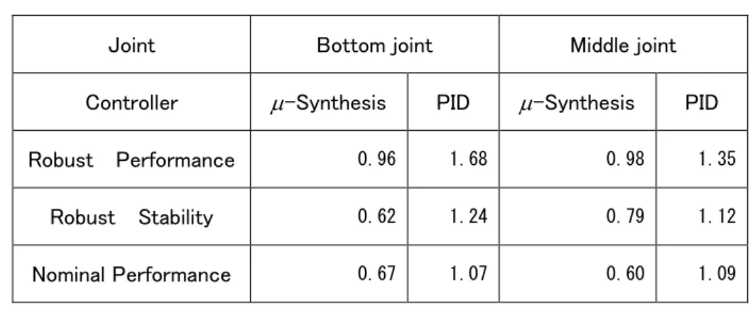
Table 3-2 Result of μ-Analysis 82

Table 3-3 PFC parameters 92

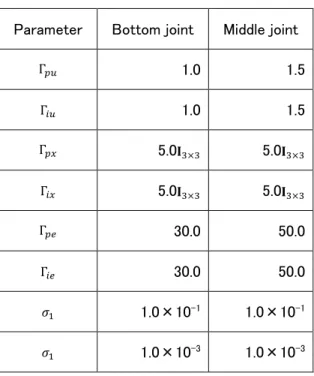
Table 3-4 SAC parameters 94

Table 3-5 SMC parameters 107

(9)

(10)

1.1 研究背景

マニピュレータというと実用化も進み，完成した技術のように感じられるが，現在でも様々な用途を目的と

して研究が盛んにおこなわれている．例えば，MIT の研究では[ 1 ]_{，従来のモータや関節といった機構ではな}

く，柔らかいボディや空気圧で変形する機構を有したアクチュエータを用いて多様な動作を可能にしたマニ

ピュレータが開発されている．ミシガン州立大学の研究では[ 2 ]_{，MEMS（Micro Electro Mechanical Systems）}

よりもさらにスケールの小さい NEMS（Nano Electro Mechanical Systems）を利用したマニピュレータが開発

(11)

第 1 章緒論 3 空気圧アクチュエータの一番の特徴は，媒体となる空気の圧縮性にある．空気の圧縮率は，油圧に比べ数千倍大きいことが知られている．オンオフ制御の場合には，この圧縮性はアクチュエータの低剛性化につながり，例えば，人が不意に装置に触れたとしても空気がクッションとなり安全性を高めることが期待できる．一方，位置や力を制御する場合には，空気の圧縮性のため，油圧や電動モータなどのアクチュエータに比べ，システムの固有周波数が低く，高周波数帯域の入力に対しては遮断特性を有するが，摩擦力など低周波数帯域の入力に対しては，その圧縮性による低剛性特性のため，制御量は影響を受けやすくなる．また，空気の圧縮性の効果が，作用する外乱の周波数帯域に応じて決定されることも制御量に影響を及ぼす原因となる．一般的に空気圧アクチュエータが高精度の制御に不向きと言われているのはこれらの影響のためである．空気圧アクチュエータの特徴を有効的に活用するためには，さまざまな用途や仕様における空気固有の振る舞いを理解することが重要性であり，近年では，エレクトロニクス技術や空気圧機器の高度化により，空気圧アクチュエータを用いたシステムにもフィードバック制御を適用した事例が多く提案されている[ 5 ]～[ 15 ]_．我々の研究室では，フルードパワーを用いた様々なデバイスの開発，設計，製作およびその制御を検討している．人や対象物を傷つけない高い構造的柔軟性を有する 3 自由度ハンド型多関節マニピュレータや 12 自由度のヒト型二足歩行ロボット，MR 流体を用いたダンパの開発など様々である[ 16 ]〜[ 25 ]_{．3 自由度ハン} ド型多関節マニピュレータは，全ての関節可動部に空気圧シリンダを組み込んだ多自由度型のシステムとなる．このマニピュレータは，空気の圧縮性による低剛性特性を利用し，柔軟に対象物へ接触し，変位または力を加え，対象物の剛性を検知するなどの用途に応用することを考えている．この際，マニピュレータの指先を所定の位置に移動，また，対象物に接触後，任意の変位や力を与える場合にはどうしてもフィードバック制御が必要となる．そのため，安定かつ制御性を向上させるためには，マニピュレータ動作時の空気の挙動を把握し，それを考慮した制御系設計手法が重要となる．

現在では，制御系設計のプロセスに，自動車業界でトレンドとなっている MBD（Model Base Design）の概

念が様々な業種で取り組まれる状況となった[ 26 ]，[ 27 ]，[ 28 ]_{．MBD は複雑化する開発業務に対し，先行開発，}

(12)

本的に開発作業を向上させる．今後の製品開発において効率的に MBD を活用することは非常に重要だと考える．

1.2 研究目的

本研究では，我々が製作した空気圧アクチュエータを用いた 3 自由度ハンド型多関節マニピュレータの位置決め制御系において，MBD により空気の圧縮性に起因する制御対象の不確かさに対し，ロバストな性能を発揮する制御系の効率的な設計手法の確立を目指す．まず，制御系設計・検証に使用するシミュレータの数式モデルやそのパラメータ同定方法について提案する．その後，位置決め制御系のロバスト化を目的としたいくつかのコントローラ設計とそれらの評価を提案したシミュレータを用いて実施する．シミュレーションにて評価した制御アルゴリズムは，自動的に C ソースコード化しハードウェアに実装して，実機にて評価をおこなう．

1.3 本論文の構成

以下に本論文の構成を示す．第 1 章緒論第 2 章マニピュレータ

第 3 章 MBD（Model Base Design）による制御系設計第 4 章実験による各コントローラの性能検証第 5 章関節間の同期を意識した制御系調整第 6 章結論

(13)

第 1 章緒論 5

第 3 章では，まず，第 2 章で算出した角度指令に対し，各関節角度が追従するためには，フィードバック制御系がどのような特性を持てば良いのかという指標を規範フィードバック制御系モデルにより評価し，相

補感度関数のバンド幅に落とし込んだ結果を示す．そして，位置制御性能を評価した PID，-Synthesis と

(14)

1.4 参考文献

[ 1 ] Girard, A, et al., “Soft Two-Degree-of-Freedom Dielectric Elastomer Position Sensor Exhibiting Linear Behavior”, IEEE/ASME Transactions on Mechatronics, Vol.20, No.1, pp.105-114(2015)

[ 2 ] Zheng Fan and Miao Yu, “Nanorobotic end-effectors: Design, fabrication, and in situ characterization”, Proceedings of the 9th IEEE International Conference on Nano/Micro Engineered and Molecular Systems, pp.6-11(2014)

[ 3 ] D.S.V. Bandra, et al., “An under-actuated mechanism for a robotic finger”, The 4th Annual IEEE International Conference on Cyber Technology in Automation, Control and Intelligent Systems, pp.407-412(2014)

[ 4 ] Kanno, T, et al., “A Forceps Manipulator With Flexible 4-DOF Mechanism for Laparoscopic Surgery”, IEEE/ASME Transactions on Mechatronics, Vol. PP, No. 99, pp.1-9(2014)

[ 5 ] 楊 , 川上 , 河合 : 摩擦力補償を用いた空気圧シリンダの位置決め制御 , 日本油空圧学会論文集 , 28-2, pp.245-251(1997) [ 6 ] 則次, 和田, 伴野 : 電空制御弁の動作遅れを考慮した空気圧サーボ系の最適制御, 計測自動制御学会論文集, 24-5, pp.490-497(1988) [ 7 ] 朝倉 , 高野 , GUO Q : 空気圧マニピュレータのロバストサーボ設計 , 日本機械学会論文集 C, 64-622, pp.2124-2131(1998) [ 8 ] 上野, 川嶋, 香川, 藤田, 榊, 菊池 : 空気圧サーボ機構における加速度フィードバック手法に関する研究, 2002 年度産業応用部門大会講演論文集(2002) [ 9 ] 小山, 密田, 原田 : 電気空気圧サーボ方式によるピストンシリンダの位置決め , 油圧と空気圧, Vol.16, No.4, pp.275-280(1985) [ 10 ] 則次, 和田 : 空気圧サーボ系の制御性能評価とその特徴, 油圧と空気圧, Vol.21, No.4, pp.417-424(1990) [ 11 ] 川村, 宮田, 花房, 石田 : 空気圧駆動システムのための階層フィードバック制御則, 計測自動制御学会論文集, Vol.26, No.2, pp.204-210(1990) [ 12 ] 宮田 , 花房 : 圧力制御を主体にした空気圧シリンダの速度制御 , 計測自動制御学会論文集 , Vol.26, No.7, pp.773-779(1990) [ 13 ] 張, 香川, 藤田, 大隅 : 静圧軸受け機構を利用した高速・精密位置決め用エアサーボテーブルの開発, 油圧と空気圧, Vol.28, No.4, pp.451-457(1997) [ 14 ] 朝倉, LI Yunsheng : むだ時間を考慮した空気圧マニピュレータの軌道追従におけるカオス現象とニューラルネットワークによる安定化制御, 日本機械学会論文集 C, 71-711, pp.3130-3137(2005) [ 15 ] 小嵜, 佐野 : ゲインスケジューリング制御を用いた空気圧サーボ系の動摩擦補償法, 日本機械学会論文集 C 編, Vol.67, No.654, pp.385-391(2001) [ 16 ] 川上 , 村山 : 研究室紹介芝浦工業大学システム理工学部川上研究室 ,油空圧技術 , Vol.55, No.8, pp.60-64(2016) [ 17 ] 村山, 川上 : 空気圧ロボットとモデルベースデザイン,油空圧技術, Vol.55, No.3, pp.23-29(2016) [ 18 ] 近藤, 村山 : 空気圧アクチュエータを用いた二足歩行ロボットの開発, 日本機械学会山梨講演会講演論文集, pp.28-29(2012) [ 19 ] 渡邉, 川上 : 空気圧アクチュエータを用いた二足歩行ロボットの開発, 日本機械学会山梨講演会講演論文集, pp.50-51(2010)

[ 20 ] Y. Kawakami, K. Ito, M. Ogawa, A. Horikawa, K.Shioda, and K. Nagai, “Development of Articulated Manipulators with Pneumatic Cylinders,” Int. J. of Automation TechnologyVol.5No.4(2011)

[ 21 ] E. Murayama, et al., “Development of new articulated manipulators with compact pneumatic cylinders”, Mechatronics and Automation (ICMA), 2012 International Conference, pp.766-771(2012)

(15)

第 1 章緒論 7 [ 27 ] 平成 23 年度モデルベース開発技術部会活動報告書 , 独立行政法人情報処理推進機構 ,

http://www.ipa.go.jp/files/000026871.pdf(2013)

(16)

(17)

(18)

2.1 ハンド型多関節マニピュレータのコンセプト

今回使用するハンド型多関節マニピュレータは，人や対象物を傷付けないための高い構造的柔軟性と，一定程度の位置制御性を目標とし設計・製作されたものである．マニピュレータの 3D CAD イメージを Fig.2-1 に示す．アクチュエータには，1)使用可能圧力範囲が広く圧力制御による力制御を行いやすいこと，2)動作方向の機械剛性は低く構造的柔軟性に優れること，3)搭載位置や搭載方法の自由度が高いこと（2)と 3)に関しては複雑な減速機構の必要がないことも利点となる），に注目し，直動複動式空気圧シリンダを採用した．

Fig.2-1 Manipulator 3D CAD image

(19)

第 2 章マニピュレータ 11

Fig.2-2 Joint mechanism

この機構を用いて，空気圧シリンダの直動運動を関節の回転運動に直接変換することで，ダイレクト駆動による正確な運動変換が可能となり，ガイドスライダを組み合わせることで，通常のガイド付きシリンダ以上に軽量かつ効果的に，シリンダ軸にかかる横荷重の対策をおこなっている．また，スライダを動かすためのスライダ軸には，摩擦抵抗軽減のためベアリングを採用し，スライダカム機構部分における軸とスライダの接触条件を滑り接触ではなく，転がり接触としている．マニピュレータには状態の計測のため感圧センサと角度センサを搭載している(Fig.2-3 参照)．各アーム内側の中間地点に力情報取得のためのアナログ式感圧センサを搭載することで，関節トルクからだけでは分からない外部の物体との接点における力の情報を利用したフルクローズド力フィードバック制御を実現可能となる．また，マニピュレータの各関節の関節軸に位置情報取得のためのアナログ式のロータリーセンサを搭載することで，関節角度を利用したフルクローズド位置フィードバック制御を実現可能となる．

(20)

2.2 ハンド型多関節マニピュレータハードウェア構成

ハンド型多関節マニピュレータ実機の写真を Fig.2-4 に示す．マニピュレータユニットは，取り付け台となるベースから根元，中間，指先関節で構成され（Fig.2-4(a)参照）， Fig.2-4(c)では対象物を把持できるように 3 つのマニピュレータユニットを組み合わせている．マニピュレータユニットの各関節には，株式会社 KOGANEI 製の小型シリンダ（Fig.2-4(b)，Table 2-1 参照）を組み込み，クランクスライダとガイドスライダを組み合わせたリンクカム機構により並進運動を関節まわりの回転運動に変換している．

(a) Top View of manipulator unit (b) Side View of Manipulator unit

(c) Assembly example of manipulator unit

Bottom Joint Middle Joint Top Joint

(21)

Table 2-1 Specifications of pneumatic cylinders

Joint Bottom Middle Top

Bore mm 15 10 10

Road Diameter mm 5 5 5

Stroke mm 20 15 15

Max. Pressure MPa 1.0 1.0 1.0

また，感圧センサについては有限会社浅草ギ研，角度センサについてはアルプス電気株式会社のものを採用した．各センサの仕様は次の通りである．

Fig.2-5 Force sensor/Pressure sensitive sensor (Asakusa Giken)

Fig.2-6 Rotary sensor (ALPS)

Table 2-2 Specifications of force sensor/pressure sensitives sensor (Asakusa Giken)

Model AS-FS

Measuring Force Range N 0 to 27.44

(22)

Table 2-3 Specifications of rotary sensor (ALPS)

Model RDC506

(23)

2.3 マニピュレータの運動学

[ 1 ]～[ 5 ]

製作したマニピュレータは 3 関節となるため，Fig.2-7 に示す 3 自由度マニピュレータの順運動学/逆運動学問題に帰着することができる．

Fig.2-7 3 degree-of-freedom manipulator

𝑥0, 𝑦0はベース（基準）座標系．𝑥𝑖, 𝑦𝑖(𝑖 = 1,2,3)は各関節におけるローカル座標系，(𝑋0, 𝑌0)はベース（基準）

座標系で表した指先の座標値を表す．また，𝑙𝑖(𝑖 = 1,2,3) m は各リンク長，𝜃𝑖(𝑖 = 1,2,3) rad は関節の角

度を表す．

このようなマニピュレータの場合，順運動学問題では Fig.2-8 のような一般化された座標系を導入し，

(24)

式（2-1）で表されるエンドエフェクタ（H）から基準座標系までの同次変換行列を求めることで，エンドエフェクタ先端の位置を基準座標系に変換している． 0 0 0 0 1 1 H H0 H 1 2 H

1

n n n 







_{ }

_





R

p

T

T T

0

（2-1）ここで，0𝐑Hは基準座標系から見たエンドエフェクタの姿勢を表す回転行列，0𝐩H0は基準座標系で表したエンドエフェクタ座標系の原点位置を表す．改めて，3 自由度マニピュレータの座標系を Fig.2-9 のように定義すると（Σ0は基準座標系，Σ𝑖(𝑖 = 1,2,3)は各関節のローカル座標系を表す），基準座標系と根元関節，根元関節と中間関節，中間関節と指先関節間の関係を表す同次変換行列0𝐓1，1𝐓2，2𝐓3は次式のように表される．

Fig.2-9 Coordinate system of 3 degree-of-freedom manipulator

(25)

第 2 章マニピュレータ 17 1 1 1 1 0 1

cos

sin

0

0 sin

cos

0

1

0

1 q

q





























T

（2- 2） 2 2 1 2 2 1 2

cos

sin

0 sin

cos

0

1

0

1 l

q





























T

（2-3） 3 3 2 3 3 1 2

cos

sin

0 sin

cos

0

1

0

1 l

q





























T

（2-4）式（2-2）～（2-4）より指先関節座標系から基準座標系までの同次変換行列0𝐓3は次のように表すことができる．















1 2 3





1 2 3



1 1 2



1 2



0 0 1 2 1 2 3 1 2 3 1 1 2 1 2 3 1 2 3

cos

sin

0 cos

cos

sin

cos

0 sin

sin

(26)

















0 1 1 2 1 2 3 1 2 3 3 0 0 e 1 1 2 1 2 3 1 2 3 3 0

cos

sin

0

1

1 X

l

Y

l

Z

q

q q

q q q

q

q q

q q q





 















_

_

_

_{ }







_{ }

_

_

 







_

_{ }















p

T

（2-7）また，指先の座標値を与えたときに式(2-7)を満たす関節角度を求める逆運動学問題に関しては，マニピュレータの指先は対象物に接触してから動作するため Fig.2-10 に示すような第 3 関節をゼロ度に固定した 2 自由度マニピュレータとして各関節角度𝜃1と𝜃2を導出した．

Fig.2-10 Geometrical relation of 2-degree-of-freedom manipulator

(27)

(28)

(29)

(30)

2.5 エンドエフェクタ移動モードの生成

2.4 章の方法で生成した指先，各関節角度の軌跡をいくつか紹介する． 2.5.1 平行移動モード平行移動モードは Fig.2-11(a)に示すように指先が XY 座標系（単位は mm）で始点位置(70,135)から終点位置(−20,135)まで 15s で移動するモードとなる．マニピュレータ全体の軌跡は Fig.2-11(b)，各関節角度の軌跡は Fig.2-11(c)となる．

(a) Trajectory interpolation in workspace of end effector

(b) Trajectory interpolation in workspace of manipulator

(c) Trajectory interpolation of manipulator joint angle Fig.2-11 Trajectory of Translation Mode

-50 0 50 100 0 20 40 60 80 100 120 140 160 Start Position. End Position.

Trajectory interpolation in workspace

Distance X [mm] D ist an c e Y [ m m ] -50 0 50 100 0 20 40 60 80 100 120 140 160 Start Position. End Position.

Distance X [mm] D ist an c e Y [ m m ] 0 5 10 15 30 35 40 45 50 55 60 65 70

75 Manipulator joint angle

(31)

2.5.2 円旋回移動モード

円旋回移動モードは Fig.2-12(a)に示すように指先が XY 座標系（単位は mm）で始点位置(50,138)から直径 35mm の円を 20s で描くモードとなる．マニピュレータ全体の軌跡は Fig.2-12(b)，各関節角度の軌跡は Fig.2-12(c)となる．

(a) Trajectory interpolation in workspace of end effector

(b) Trajectory interpolation in workspace of manipulator

(c) Trajectory interpolation of manipulator joint angle Fig.2-12 Trajectory of Circular Mode

以下，これらの移動モードに対応した各関節角度の軌跡を目標角度として入力し，シミュレーションと実験により指先の位置制御性能の検証をおこなう． -50 0 50 100 150 0 20 40 60 80 100 120 140 160 Start Position. End Position.

Distance X [mm] D ist an c e Y [ m m ] -50 0 50 100 0 20 40 60 80 100 120 140 160 Start Position. End Position. Trajectory interpolation in workspace

Distance X [mm] D ist an c e Y [ m m ] 0 5 10 15 20 20 30 40 50 60 70 80

90 Manipulator joint angle

(32)

2.6 実験機構成

Fig.2-13 に実験装置の概略を示す．各関節の角度指令とコントローラは Host PC にインストールされた

MATLAB/Simulink®_{上で設計し，xPC-Target™を用いてリアルタイム OS 用のアプリケーションを作成して，}

LAN 経由で Target PC に実装する．Target PC では実装されたアプリケーションによりマニピュレータの制御とデータの計測をおこなう．実験終了後，計測したデータは LAN 経由で Host PC に転送される．

Fig.2-13 Hardware configurations

(33)

第 2 章マニピュレータ 25 また，電空レギュレータの電圧・圧力変換式（校正値）は次式となる．

0.9 0.001

0.001 0.0899

0.001 10 0

P





V





V





（2-29）ここで𝑃は電空レギュレータ圧力 MPa，𝑉は指令電圧 V となる．

Fig.2-14 Electro-pneumatic regulator characteristic Table 2-4 Specifications of electro-pneumatic regulator (SMC)

Model ITV0051-3MS

Min. Supply Pressure MPa Set pressure + 0.1

Max. Supply Pressure MPa 1.0

Set Pressure Range MPa 0.001 to 0.9

Max. Flow Rate l/min 6

Voltage [V]

Pressure [MPa]

0.9

0.001

(34)

2.7 システム同定と制御対象ノミナルモデル

MBD（Model Base Design）ベースで制御系の設計・検討をおこなう場合，コントローラ設計用のノミナルモデルや実験機のシミュレータが必要となる．この章では，非線形摩擦を含む実験機シミュレータの構築とシステム同定，ノミナルモデルの算出について説明する．

2.7.1 空気圧サーボシステムの数学モデル

空気圧シリンダとクランクスライダとガイドスライダを組み合わせたリンクカム機構の概略図を Fig.2-15 に示す．

Fig.2-15 Pneumatic cylinder and link-cam mechanism

(35)

(36)

(37)

第 2 章マニピュレータ 29 式（2-39）は次のように書き表せる．

 

1 2 2 3 6 ep ep H ep 3 1 2 3 ep ep ep ep

10 x t

x t

D

K T

J

D T

L A

K

x t

u t

J T







_





_{ }

_

_



_{ }

_

_



_



（2-42）ここで，出力𝑦(𝑡)を関節角度𝜃(𝑡)とすると，関節リンク回転運動の状態方程式は式（2-43）のように表すことができる．

 





 

1 1 2 2 3 3 6 ep ep H ep ep ep ep ep 1 2 3 0 0 1 0 0 0 1 0 10 1 0 0 x t x t d x t x t u t dt x t x t D K T J D T L A K K J T J T J T J T x t y t x t x t            _ _  _ _    _ _  _ _    _ _ _ _   _ _  _ _           _{ } _{ }          _ _ _      _ _ _  _       _ _  _ _   _ _  _ _     （2-43） 2.7.2 周波数応答実験マニピュレータの特性を調べるために周波数応答実験をおこなった．マニピュレータの根元関節と中間関節に組み込まれた空気圧シリンダに対し，開ループシステムでは，周期的な入力信号に対して中立点がずれていき，出力がうまく計測できないため，PI コントローラにより制御量を関節角度としたフィードバック系を構成して，動作圧力については，ロッド側に 0.36MPa（指令電圧 4V 相当），ヘッド側に受圧面積比を掛けた 0.27MPa を設定し，45deg までステップ応答により関節角度を振り上げ，その角度から 30deg 振幅の対数チャープ信号と M 系列信号を入力し周波数応答を計測する．N 増し回数は 5 回とした．

また，閉ループシステムの計測結果に対し，周波数解析後に相補感度関数のゲイン・位相特性が得られるが，それを数式処理し，一巡伝達関数，制御対象のゲイン・位相特性もあわせて算出した．

(38)

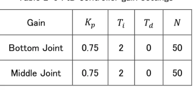
Table 2-5 PID controller gain settings Gain 𝐾𝑝 𝑇𝑖 𝑇𝑑 𝑁 Bottom Joint 0.75 2 0 50 Middle Joint 0.75 2 0 50 Fig.2-16(a)に対数チャープ信号による計測結果（根元関節）と Fig.2-16(b)にコヒーレンスを示す． Fig.2-16(a)から，動き出しと速度が反転する部分でスティックスリップの影響と思われる振動が見られる．また 0.1～1Hz でコヒーレンスの値が落ち着いていないのもこの振動が原因だと思われる．

(a) Log-swept chirp signals

(b) Coherence

Fig.2-16 Bottom joint frequency response experiments

(39)

Fig.2-17 に Fig.2-16(a)を周波数解析して算出したゲイン・位相特性を示す．

Fig.2-17(f)から低い周波数帯域で約-90deg と制御対象の位相遅れが大きいことがわかる．これはスティックスリップにより動きだしに遅れが生じたことが原因だと思われる．

(a) Complementary sensitivity function : Gain (b) Complementary sensitivity function : Phase

(c) Loop transfer function : Gain (d) Loop transfer function : Phase

(e) Plant : Gain (f) Plant Phase

Fig.2-17 Bottom joint frequency analysis (Log-swept chirp signals)

(40)

Fig.2-18(a)に M 系列信号による計測結果（根元関節）と Fig.2-18(b)にコヒーレンスを示す．

コヒーレンスが低周波数帯域で 1 近傍に落ち着いていることから相関の良い計測結果であることがわかる．

(a) M-Sequence signals

(b) Coherence

Fig.2-18 Bottom joint frequency response experiments

(41)

Fig.2-19 に Fig.2-18(a)を周波数解析して算出したゲイン・位相特性を示す．

Fig.2-19(f)から低い周波数帯域で約 0deg と制御対象の位相遅れがほぼないことがわかる．

(a) Complementary sensitivity function : Gain (b) Complementary sensitivity function : Phase

(c) Loop transfer function : Gain (d) Loop transfer function : Phase

(e) Plant : Gain (f) Plant Phase

Fig.2-19 Bottom joint frequency analysis (M-Sequence signals)

(42)

(43)

Fig.2-20 LuGre friction model

以上から，制御対象のモデルは Fig.2-21 のように構成した．LuGre 摩擦モデルに加え，電空レギュレータの

むだ時間𝑇𝑑𝑙𝑦と調整用ゲイン𝐾𝑚𝑑𝑙を追加している．

Fig.2-21 Plant model

𝐾𝑚𝑑𝑙はシステム構成要素のカタログスペックからのばらつきなどを調整するために導入したゲインである．この変更により，制御対象は次のような伝達関数と状態方程式で記述される．

 

_{ }

_

mdl H

_

ep 6

_

n ₂ MV ep

10

1 K

L A

K

s

P s

V

s

Js

Ds

K

T s

q

 









（2-46） T[Nm] [rad/s] FS FC -FC -FS D 1 ep ep K T s  PH[MPa] 106 PH[Pa] _K mdl AH L F [N] T [Nm] －－＋－ 1/J 1 s     vs sgn  ss C S C T F F F e   _    _    D K 1 s  [rad/s] q [rad] VMV[V]

Nonlinear Friction Torque[Nm]

Viscous Torque[Nm]

Elastic Torque[Nm]

dly

T s

(44)

(45)

Table 2-6 Result of system identification

No Design Variables Bottom Joint Middle Joint

1 Kmdl 1.034E+00 1.007E+00

2 L 5.166E-02 7.867E-02

3 J 5.680E-04 7.660E-04

4 D 1.880E-01 2.390E-01

5 K 1.740E-02 1.315E-02

6 Tep 4.371E-02 4.277E-02

7 Tdly 8.117E-02 3.941E-02

8 Fs 2.664E-01 2.200E-01

9 Fc 8.918E-02 7.371E-02

10 vs 9.919E-02 5.794E-02

11 alpha 1.961E+00 1.966E+00

12 beta 1.683E+00 1.737E+00

最適化アルゴリズムには DE（Differential Evolution）を採用した．DE は，連続変数を対象とした関数の勾配を用いない多点同時探索型最適化手法の一つで，突然変異，交叉，適者生存という操作を繰り返しながら，大域的最適解を求める方法である．GA（Genetic Algorithm，遺伝的アルゴリズム）の考え方に強い影響を受けた手法であると思われ，メタヒューリスティックの一つとして考えることができる．探索個体 40，イテレーション 1500，低周波数正弦波に関する評価関数重み係数 2.0，M 系列に関する評価関数重み係数 0.5 の設定で最適化した際の同定結果を Table 2-6 に示す．計算時間は CPU: インテル®

(46)

(a) Modeling result : Low frequency sine wave (b) Verification result : Low frequency sine wave

(c) Modeling result : M-Sequence signals (d) Verification result : M-Sequence signals

(e) Plant gain (f) Plant phase

Fig.2-22 Comparison between experiment and simulation of bottom joint

Fig.2-23 Friction characteristic bottom joint

(47)

(a) Modeling result : Low frequency sine wave (b) Verification result : Low frequency sine wave

(c) Modeling result : M-Sequence signals (d) Verification result : M-Sequence signals

(e) Plant gain (f) Plant phase

Fig.2-24 Comparison between experiment and simulation of middle joint

Fig.2-25 Friction characteristic middle joint

(48)

(49)

(50)

また，線形チャープ信号，対数チャープ信号を入力し，その実験結果から算出した周波数特性は，さらにばらつきが大きいことがわかる．そこで，次のような伝達関数を導入し，

 

_

_

_

dly 6 min tune mdl H ep min 2 ep

10

1

T s

K

L A

K

P

s

e

Js

Ds

K

T s

 



 









（2-53）

 

_

_

_

dly 6 max tune mdl H ep max 2 ep

10

1

T s

K

L A

K

P

s

e

Js

Ds

K

T s

 



 









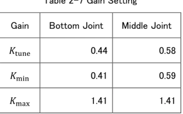
（2-54）ゲイン𝐾min，𝐾maxとむだ時間要素により，不確かさの最大・最小を見積もった．ただし，むだ時間は 8 次のパデ近似でモデル化する．

ゲイン𝐾tune，𝐾min，𝐾maxは Table 2-7 のように決定した．また，このときの周波数特性を Fig.2-26 と

Fig.2-27 に重ねてプロットした．

Table 2-7 Gain Setting

Gain Bottom Joint Middle Joint

𝐾tune 0.44 0.58

𝐾min 0.41 0.59

𝐾max 1.41 1.41

(51)

(a) Plant gain

(b) Plant phase

Fig.2-26 Bottom joint frequency characteristic

10-1 100 101 -100 -50 0 50 根元関節ゲイン特性不確かさ Frequency [Hz] G ai n [ dB ] Nominal

Gain Min+Dead Time Element Gain Max+Dead Time Element

10-1 100 101 -200 -150 -100 -50 0 50 100 150 200 根元関節位相特性不確かさ Frequency [Hz] Ph ase [ de g] Nominal

(52)

(a) Plant gain

(b) Plant phase

Fig.2-27 Middle joint frequency characteristic

10-1 100 101 -100 -50 0 50 中間関節ゲイン特性不確かさ Frequency [Hz] G ai n [ dB ] Nominal

Gain Min+Dead Time Element Gain Max+Dead Time Element

10-1 100 101 -200 -150 -100 -50 0 50 100 150 200 中間関節位相特性不確かさ Frequency [Hz] Ph ase [ de g] Nominal

(53)

2.8 参考文献

○マニピュレータ

[ 1 ] 澤田, 板宮 : 計算トルク法をベースとしたロボットアームの適応軌道制御系の過渡応答改善法-滑らかな射影アルゴリズムの利用-, 計測自動制御学会論文集, Vol.10, No.7, pp.58-65(2011)

[ 2 ] Richard M. Murray, “A Mathematical Introduction to Robotic Manipulation”, CRC Press(1994)

[ 3 ] 小坂, 島田 : モータと減速機を考慮したロボットマニピュレータ制御, 計測自動制御学会論文集, Vol.41, No.5, pp.466-472(2005) [ 4 ] 川嶋, 只野 : 絵ときでわかるロボット工学（第 2 版）, オーム社(2014) [ 5 ] 吉川 : ロボット制御基礎論, コロナ社(1988) ○空気圧システムのモデル化 [ 6 ] 木村, 藤田, 原, 香川 : 厳密な線形化を用いた空気圧アクチュエータ駆動系の制御, システム制御情報学会論文誌, Vol.8, No.2, pp.52-60(1995) [ 7 ] 花房 : サーボ系における非線形特性の処理, 計測と制御, Vol.17, No.7, pp.514-522(1978) [ 8 ] 山藤 : 空気圧アクチュエータのロボット制御への応用, 日本ロボット学会誌, Vol.9, No.4, pp.498-501(1991) [ 9 ] 電空制御弁の動作遅れを考慮した空気圧サーボ系の最適制御, 計測自動制御学会論文集, Vol.24, No.5, pp.490-497(1988) [ 10 ] 高岩, 則次 : 空気式パラレルマニピュレータを用いた手首部リハビリ支援装置の開発-多自由度リハビリ動作の実現-, 日本ロボット学会誌, Vol.24, No.6, pp.747-753(2006) [ 11 ] 朝倉, 高野, 国 : 空気圧マニピュレータのロバストサーボ設計, 日本機械学会論文集（C 編）, Vol.64, No.622, pp.2124-2131(1998) [ 12 ] 辻内, 小泉, 西野, 小松原, 久田原, 平野 : 空気圧駆動マスタ・スレーブハンドの開発と関節制御, 日本機械学会論文集（C 編）, Vol.74, No.741, pp.1267-1272(2008) [ 13 ] 川上, 野口, 河合 : 空気圧シリンダの高速駆動に関する一考察, 油圧と空気圧, Vol.21, No.3, pp.318-325(1990) [ 14 ] 川上, 武田, 河合 : 空気圧シリンダの駆動条件に関する一考察, 油圧と空気圧, Vol.22, No.4, pp.452-459(1991) [ 15 ] 木村 : MATRIXx を用いた空気圧系の実践的ロバスト制御系設計, 日本フルードパワーシステム学会講習会資料(1999) [ 16 ] 藤沼 : 空気圧サーボによる位置制御の研究, 茨城県工業技術センター研究報告, No.16, pp.9-13(1987) [ 17 ] 松浦, 新谷 : モデルベースド制御による空気圧駆動マニピュレータの位置決め制御, システム制御情報学会論文誌, Vol.5, No.10, pp.410-417(1992)

[ 18 ] Bashir M. Y. Nouri, et al., “MODELLING A PNEUMATIC SERVO POSITIONING SYSTEM WITH FRICTION”, Proceedings of the American Control Conference, pp.1067-1071(2000)

[ 19 ] J.Wang, D.J.D.Wang, P.R.Moore and J.Pu, “Modelling study, analysis and robust servocontrol of pneumatic cylinder actuator systems”, IEE Proc.-Control Theory Appl., Vol.148, No.1, pp.35-42(2001)

[ 20 ] Shu Ning and Gary M. Bone, “Development of a Nonlinear Dynamic Model for a Servo Pneumatic Positioning System”, Proceedings of the IEEE International Conference on Mechatronics & Automation, pp.43-48(2005)

[ 21 ] Wang Bo, Wang Tao, Jin Ying, Fan Wei and Wang Yu, “Study of Pneumatic Servo System Based on Linear Active Disturbance Rejection Controller”, 2013 IEEE/ASME International Conference on Advanced Intelligent Mechatronics (AIM), pp.1170-1174(2013)

○非線形摩擦

[ 22 ] 小嵜, 佐野, 香川 : 空気圧駆動系におけるスティックスリップの発生限界, 日本機械学会論文集（C 編）, Vol.68, No.669, pp.1363-1370(2002)

[ 23 ] Owen, W.S. and Croft, E.A., "The reduction of stick-slip friction in hydraulic actuators", Mechatronics, IEEE/ASME Transactions, Vol.8, No.3, pp.362-371(2003)

[ 24 ] Sami Moisio, et al., "Simulation of tactile sensors using soft contacts for robot grasping applications", Robotics and Automation (ICRA), 2012 IEEE International Conference, pp.5037-5043(2012)

[ 25 ] Marton, L. and Lantos, B., "Modeling, Identification, and Compensation of Stick-Slip Friction" , Industrial Electronics, IEEE Transactions , Vol.54 , No.1, pp.511-521(2007)

[ 26 ] Johanastrom, K. and Canudas-de-Wit, "Revisiting the LuGre friction model", Control Systems, IEEE, Vol.28, No.6, pp.101-114(2008)

(54)

[ 28 ] Radcliffe, Clark J. and Southward, Steve C., "A Property of Stick-Slip Friction Models which Promotes Limit Cycle Generation", American Control Conference, pp.1198-1205(1990)

[ 29 ] Matej, P. and Makys, P., "Influence of static friction and stick-slip phenomena on control quality of SMPM", ELEKTRO, pp.232-235(2012) ○同定 [ 30 ] 加藤, 左近, 山本, 大川 : 宇宙用マニピュレータのパラメータ同定と手先軌道制御, 日本機械学会論文集（C 編）, Vol.61, No.585, pp.1974-1980(1995) [ 31 ] 藤本, 田中, 川上 : 平面マニピュレータの機構パラメータ同定に関する一考察, 電子情報通信学会技術研究報告. NLP, 非線形問題, Vol.99, No.134, pp.91-97(1999) [ 32 ] 豊澤, 園田, 原田, 柏木 : 非線形摩擦を含む共振系機械モデルのオンライン同定 (第 1 報)—実用的なオンライン同定法の開発—, 精密工学会誌, VOl.78, No.6, pp.488-493(2012) [ 33 ] 豊澤, 園田, 原田, 柏木 : 非線形摩擦を含む共振系機械モデルのオンライン同定 (第 2 報)—2 慣性系の機械パラメータをオンラインで同定する実用的な方法—, 精密工学会誌, VOl.78, No.12, pp.1093-1098(2012) ○最適化アルゴリズム DE(Differential Evolution)

[ 34 ] Differential Evolution (DE) for Continuous Function Optimization, https://jp.mathworks.com/matlabcentral/linkexchange/links/24

[ 35 ] Differential Evolution (DE) for Continuous Function Optimization (an algorithm by Kenneth Price and Rainer Storn), http://www1.icsi.berkeley.edu/~storn/code.html

[ 36 ] 北山, 酒井, 荒川, 山﨑 : 大域的最適化法としての Differential Evolution と数値計算, 日本機械学会論文集 C 編, Vol.76, No.771, pp.2819-2828(2010)

(55)

(56)

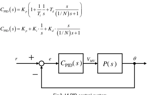
3.1 規範フィードバック制御系モデルによるエンドエフェクタ位置，関節角度追従性の確認

各関節の制御系は Fig.3-1 のようなフィードバック制御系となるため，目標角度 r から関節角度までの伝

達関数を𝐺FB(𝑠)とおくと式（3-1）のように表される．

Fig.3-1 Feedback control system

 

_{ }

FB

 

_{ }

FB FB

1 P s C

s

G

s

P s C

s





（3-1）ここで，𝑃(𝑠)は実機または非線形摩擦を含む制御対象モデル，𝐶FB(𝑠)はフィードバックコントローラを表す．このとき関節角度の追従性は式（3-1）の伝達関数の周波数特性に依存し，設計者は希望する周波数特性に合致するような𝐶FB(𝑠)を検討しなければならない．本研究では，PID をはじめ，-Synthesis，SAC(Simple

(57)

第 3 章 MBD(Model Base Design)による制御系設計 49 再現できること，代表根を空気の圧縮性や関節回転系の周波数特性と見れば，おそらく低次で特性が再現できることを考慮して，このモデルを採用した．この規範フィードバック制御系モデルに前章で設計した平行移動モードと円旋回移動モードの各関節角度指令を入力し，その関節角度応答と誤差，順運動学により算出した指先軌跡誤差と規範フィードバック制御系モデルのバンド幅を整理する．固有振動数𝜔𝑛は 0.5，1.0，1.5，1.8Hz とし，バンド幅の影響のみを知りたいため，減衰係数ζは 1 として，オーバーシュートが発生しないようにした． Fig.3-2 に固有振動数𝜔𝑛を 0.5，1.0，1.5，1.8Hz としたときの規範フィードバック制御系モデルのゲイン特性を示す．また，Fig.3-3～Fig.3-10 にシミュレーション結果を示す．

Fig.3-2 Gain characteristics of reference feedback model

10

-2

10

-1

10

0

10

1

10

2

-10

-8

-6

-4

-2

0

2 Reference Feedback Model

(58)

(a) Gain characteristics (b) End effector trajectory

(c) Joint trajectory of bottom (d) Joint trajectory of middle

(e) Joint error of bottom (f) Joint error of middle

Fig.3-3 Simulation of translation mode: 𝜔𝑛= 0.5Hz

10-2 10-1 100 101 102 -10 -8 -6 -4 -2 0

2 Reference Feedback Model for Bottom Joint

Frequency [Hz] G ai n [ dB ] 0 20 40 60 80 100 120 140 80 90 100 110 120 130 140 150 Start Position. End Position.

Distance X [mm] D ist an c e Y [ m m ] Reference Response 2 4 6 8 10 12 14 16 0 10 20 30 40 50

60 Bottom Joint Angle Response

Time [s] A n gl e [ de g] Reference

Reference Feedback Model

2 4 6 8 10 12 14 16 0 20 40 60 80

100 Middle Joint Angle Response

2 4 6 8 10 12 14 16 -6 -4 -2 0 2 4

6 Bottom Joint Angle Error

Time [s] A n gl e [ de g] 2 4 6 8 10 12 14 16 -4 -2 0 2 4 6 8

10 Middle Joint Angle Error

(59)

第 3 章 MBD(Model Base Design)による制御系設計 51

10-2 10-1 100 101 102 -10 -8 -6 -4 -2 0

2 4 6 8 10 12 14 16 0 20 40 60 80

2 4 6 8 10 12 14 16 -3 -2 -1 0 1 2

Time [s] A n gl e [ de g] 2 4 6 8 10 12 14 16 -2 -1 0 1 2 3 4

(60)

10-2 10-1 100 101 102 -10 -8 -6 -4 -2 0

2 4 6 8 10 12 14 16 0 20 40 60 80

2 4 6 8 10 12 14 16

-2 -1 0 1

Time [s] A n gl e [ de g] 2 4 6 8 10 12 14 16 -2 -1 0 1 2 3

(61)

10-2 10-1 100 101 102 -10 -8 -6 -4 -2 0

2 4 6 8 10 12 14 16 0 20 40 60 80

2 4 6 8 10 12 14 16

-2 -1 0 1

Time [s] A n gl e [ de g] 2 4 6 8 10 12 14 16 -1 0 1 2

(62)

Fig.3-7 Simulation of circular mode: 𝜔𝑛 = 0.5Hz

10-2 10-1 100 101 102 -10 -8 -6 -4 -2 0

Frequency [Hz] G ai n [ dB ] 0 20 40 60 80 110 120 130 140 150 Start Position. End Position. Trajectory interpolation in workspace

Distance X [mm] D ist an c e Y [ m m ] Reference Response 5 10 15 20 0 10 20 30 40 50 60

5 10 15 20

20 40 60 80

5 10 15 20 -6 -4 -2 0 2 4

Time [s] A n gl e [ de g] 5 10 15 20 -10 -5 0 5

(63)

10-2 10-1 100 101 102 -10 -8 -6 -4 -2 0

5 10 15 20

20 40 60 80

5 10 15 20 -3 -2 -1 0 1 2

Time [s] A n gl e [ de g] 5 10 15 20 -4 -2 0 2

(64)

10-2 10-1 100 101 102 -10 -8 -6 -4 -2 0

5 10 15 20

20 40 60 80

5 10 15 20 -1.5 -1 -0.5 0 0.5 1 1.5

Time [s] A n gl e [ de g] 5 10 15 20 -3 -2 -1 0 1 2

(65)

10-2 10-1 100 101 102 -10 -8 -6 -4 -2 0

5 10 15 20

20 40 60 80

5 10 15 20 -1.5 -1 -0.5 0 0.5 1

1.5 Bottom Joint Angle Error

Time [s] A n gl e [ de g] 5 10 15 20 -2 -1 0 1

(66)

以上のシミュレーション結果から，固有振動数𝜔𝑛を 0.5，1.0，1.5，1.8Hz としたときの規範フィードバック

制御系のバンド幅を Fig.3-11 に示す．また各モードの誤差解析結果を Fig.3-12，Fig.3-13 に示す．

Fig.3-11 Bandwidth of reference feedback model

(a) Error of Joint (b) Error of end effector

Fig.3-12 Error analysis of translation mode

(a) Error of Joint (b) Error of end effector

(67)

Fig.3-3～Fig.3-10 のグラフでマーカーは誤差が最大となっている位置を示している．Fig.3-12 と Fig.3-13 で「+方向誤差」とは，角度指令に対し角度応答との偏差が 0 より大きいときの最大誤差，「-方向誤差」とは，偏差が 0 より小さいときの最大誤差を示している．

(68)

3.2 PID 制御

PID コントローラは式（3-3），（3-4）で表されるもので，Simulink には式（3-4）のパラレル型の形式で実装した．SILS 用モデルは，Fig.3-14 のブロック線図の構成で実装し，𝑃(𝑠)には非線形摩擦モデルを含む制御対象モデルを使用している．

 

_

_

PID

1 1

1 1/

1

p d i

s

C

s

K

T

T s

N s









_





_







（3-3）

 

_

_

PID

1 1/

1

p i d

s

C

s

K

s

N s





 





（3-4）

Fig.3-14 PID control system

今回使用した PID コントローラのゲインは Table 3-1 となる．両関節ともシステム同定に使用した比例ゲイン 0.75 から上げて，また根元関節については積分時間を 2.0 から 1.3 まで下げ，角度偏差に対する操作量を増加させている．

Table 3-1 PID controller gain settings

(69)

(70)

(a) Log-swept chirp signals of bottom joint (b) Log-swept chirp signals of middle joint

(c) Coherence of bottom joint (d) Coherence of middle joint

Fig.3-15 Frequency response simulation: PID

(a) Bottom joint (b) Middle joint

(71)

(a) Complementary sensitivity function of bottom joint (b) Complementary sensitivity function of middle joint

(c) Sensitivity function of bottom joint (d) Sensitivity function of middle joint

Fig.3-17 Frequency analysis of complementary sensitivity function and sensitivity function: PID

(a) Bottom joint (b) Middle joint

Fig.3-18 Step response simulation: PID

多自由度空気圧シリンダシステムの制御系設計手法に関する研究

学位論文題目