円制限三体問題における宇宙機の運動の設計と制御

円制限三体問題における宇宙機の運動の設計と制御

秋山, 祐貴

https://doi.org/10.15017/1931914

出版情報：Kyushu University, 2017, 博士（工学）, 課程博士 バージョン：

権利関係：

Design and Control of Spacecraft Motion in Circular Restricted Three-Body Problem

A dissertation submitted in partial fulfillment of the requirements for the degree of Doctor of Philosophy

Department of Aeronautics and Astronautics Kyushu University

Japan

Yuki Akiyama

2018

ACKNOWLEDGMENT

My heartfelt appreciation goes to my supervisor, Associate Professor Mai Bando, for her expert guidance, generous support and encouragement throughout my student life. Discussions with her always led me to find novel ideas and to think from different points of view. I would not have completed this dissertation without her kind help and guidance.

I would like to thank Professor Shinji Hokamoto, whose comments about and suggestions for my study proved inestimably valuable. His great advice about my research and career was both helpful and wise.

I am grateful to Professor Kenji Fujimoto from Kyoto University and Professor Yasuhiro Kawakatsu from Institute of Space and Astronautical Science, Japan Aerospace Exploration Agency (ISAS/JAXA) for their pointed questions, arguments, and great efforts to patiently correct, improve, and finalize this dissertation.

Special thanks go to the members of the Guidance and Control Laboratory (GCL). I have been in GCL for five years including one year of Bachelor’s course period and two years of Master course period. All the people I met in GCL made my research life wonderful and productive.

I also would like to express my gratitude to my family members for their extraordinary love, moral support and warm encouragement.

Finally, I owe thanks to the Japan Society for the Promotion of Science (JSPS) for its generous provision of financial assistance. The work in this dissertation was supported in part by JSPS KAKENHI（Grants-in-Aid for Scientific Research) Grant Number JP17J02998.

i

ACKNOWLEDGMENT i

LIST OF FIGURES x

LIST OF TABLES xi

LIST OF PARAMETERS xii

I INTRODUCTION AND PRELIMINARIES 1

1 Introduction 2

1.1 Background . . . 2

1.2 Research Objectives . . . 8

1.2.1 Development of trajectory design methods . . . 8

1.2.2 Development of control methods . . . 9

1.3 Dissertation Overview . . . 10

2 Preliminaries 12 2.1 Restricted Three-Body Problem . . . 12

2.2 Circular Restricted Three-Body Problem . . . 13

2.2.1 Equation of motion . . . 13

2.2.2 Libration points . . . 16

2.2.3 Variational equations . . . 18 ii

CONTENTS iii

2.2.4 Periodic orbits . . . 20

2.2.5 Invariant manifolds . . . 21

2.3 Attitude Dynamics . . . 25

2.3.1 Rotational kinematics . . . 26

2.3.2 Kinematic differential equations . . . 30

2.3.3 Dynamics differential equations . . . 30

2.4 Center manifold theory . . . 31

2.5 Output Regulation Theory for Nonlinear Systems . . . 32

2.5.1 System equations and basic assumptions . . . 33

2.5.2 Nonlinear local output regulation problem . . . 34

2.5.3 Solvability of the nonlinear local output regulation problem . . . 35

II LOW-THRUST TRAJECTORY DESIGN 37

3.1.1 Derivation of divided form of the CRTBP dynamics . . . 39

3.1.2 Finding the center manifold of the CRTBP . . . 42

3.2 Center Manifold Design Method for Periodic Orbits . . . 44

3.2.1 State transition matrix . . . 44

3.2.2 Deviation of initial state . . . 45

3.3 Simulation for Sun-Earth CRTBP . . . 47

3.3.1 Verification of the center manifold design method . . . 47

3.3.2 Physical meaning of the parameter vector . . . 49

3.3.3 Family of Lyapunov orbits . . . 51

3.3.4 Finding vertical Lyapunov orbit from quasi-periodic orbit around L₁ . . 52

3.3.5 Finding halo orbit from quasi-periodic orbit around L₂ . . . 54

3.4 Summary . . . 56

4 Invariant Manifolds Design Under Low-Thrust Control Acceleration 60

4.1 Natural and Artificial Invariant Manifolds . . . 60

4.1.1 Eigenstructures of natural system and artificial system . . . 60

4.1.2 General expression for control acceleration . . . 62

4.1.3 Design of natural and artificial periodic orbits . . . 63

4.1.4 Definition of natural and artificial manifolds . . . 64

4.2 Examples of Artificial Periodic Orbits and Artificial Invariant Manifolds . . . . 65

4.2.1 Zeroth-order effect . . . 66

4.2.2 First-order effect . . . 69

4.3 Summary . . . 76

III CONTROL STRATEGY BASED ON OUTPUT REGULATION THEORY 77

5.1.1 Exact tracking controller . . . 79

5.1.2 Approximated tracking controller . . . 81

5.2 Formation Flying Strategy . . . 84

5.3 Simulation for Sun-Earth L₂Point . . . 87

5.3.1 Station-keeping on libration orbits . . . 90

5.3.2 Performance indices of station-keeping . . . 91

5.3.3 Formation flying along a Lyapunov orbit . . . 96

5.3.4 Formation flying along a halo orbit . . . 98

5.3.5 Effects of Perturbations on the Proposed Controller . . . 99

5.4 Summary . . . 102

CONTENTS v 6 Orbit-Attitude Control Based on Nonlinear Output Regulation Theory 104

6.1 Coupled Orbit-Attitude Dynamics in the CRTBP . . . 104

6.1.1 Problem assumptions and coordinate frames . . . 104

6.1.2 Orbital dynamics . . . 105

6.1.3 Gravity gradient torque in the CRTBP . . . 106

6.1.4 Attitude dynamics . . . 107

6.1.5 State space form . . . 109

6.2 Orbit-Attitude Control Strategy . . . 110

6.2.1 Orbit-attitude controller . . . 110

6.2.2 Determination of feedback gain . . . 115

6.3 Simulation for Sun-Earth L₂Point . . . 117

6.3.1 Station-keeping on libration point orbits with constant attitude . . . 119

6.3.2 Station-keeping on libration point orbits with periodic attitude . . . 122

6.3.3 Station-keeping cost . . . 124

6.3.4 Orbit-attitude control with thrusters . . . 124

6.4 Summary . . . 127

IV CONCLUSION 129

7.1.1 Development of trajectory design methods . . . 130

7.1.2 Development of control methods . . . 131

7.2 Recommendations for Future Work . . . 132

7.2.1 Development of trajectory design methods . . . 132

7.2.2 Development of control methods . . . 134

REFERENCES 136

APPENDICES 148

A Stability Analysis 149

A.1 Orbital Stability . . . 149

A.1.1 Stability of the out-of-plane motion . . . 149

A.1.2 Stability of the in-plane motion . . . 150

A.1.3 Summary of Stability . . . 154

A.2 Attitude Stability on Collinear Lagrangian Points . . . 154

B Derivations of Equation (3.28) 159 C Proofs of Properties of Derived Controllers 161 C.1 Relation Between Truncation Order and Performance Index for Control Input Given by (5.27) . . . 161

C.2 Relation Between Controllers (5.13) and (5.27) . . . 163

C.3 Relation Between Truncation Order and Performance Index for Control Acceleration Given in (6.63) . . . 163

LIST OF FIGURES

2.1 Circular restricted three-body system with two reference frames: inertial frame ( ˆI-frame) and rotational frame ( ˆr-frame). . . . 13 2.2 Configuration of Lagrangian points. . . 16 2.3 Lyapunov orbits around Sun-Earth L₁ point: the symbol ∗ denotes L₁

Lagrangian point. . . 21 2.4 Halo orbits around Sun-Earth L₁point: the blue and red orbits denotes northern

and southern halo orbits, respectively; the symbol∗denotes the L₁Lagrangian point. . . 22 2.5 Invariant manifolds associated with the Sun-Earth L₁ point: the symbol ∗ is

denotes L₁ Lagrangian point; the blue and red lines denote the stable and unstable manifolds, respectively. . . 23 2.6 Invariant manifolds associated with the Sun-Earth L₁Lyapunov orbit: the blue

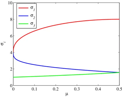
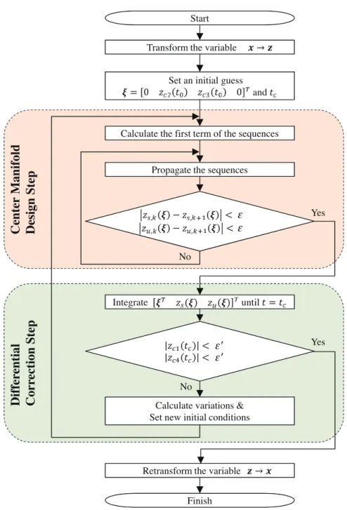
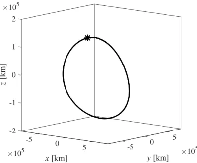
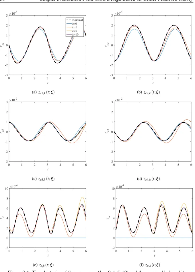
and red tube-like structures denote the stable and unstable manifolds, respectively. 24 3.1 Relation betweenµ ^andσi. . . 40 3.2 Flowchart of center manifold design method for periodic orbits. . . 48 3.3 Nominal halo orbit. . . 49 3.4 Time histories of the sequences (k=0,1,5,10) and the nominal halo orbit. . . . 50 3.5 Quasi-periodic orbit (quasi-vertical Lyapunov orbit): ξ = [1,0,0,0]^T×10⁻².

The initial positions are shown by asterisks. . . 51 vii

3.6 Quasi-periodic orbit (quasi-vertical Lyapunov orbit): ξ = [0,1,0,0]^T×10⁻². The initial positions are shown by asterisks. . . 52 3.7 Periodic orbits (Lyapunov orbits): ξ = [0,0,z_c3(t₀),z_c4(t₀)]^T. The initial

positions are shown by asterisks. . . 53 3.8 Lyapunov families obtained by the center manifold design method. . . 53 3.9 Periodic orbit obtained by differential correction step (zc₂-fixed case). The

red and blue orbits are obtained by the center manifold step and differential correction step, respectively. The initial positions are shown by asterisks. . . . 55 3.10 Periodic orbit obtained by differential correction step (z_c2-fixed case). The

red and blue orbits are obtained by the center manifold step and differential correction step, respectively. The initial positions are shown by asterisks. . . . 57 3.11 Periodic orbit by differential correction step (zc₃-fixed case). The red and blue

orbits are obtained by the center manifold step and differential correction step, respectively. The initial positions are shown by asterisks. . . 58 4.1 NPO and APOs (ξ3=0.8×10⁻²): the solid lines represent the obtained orbits,

the dashed lines represent the NPO, the black asterisks at the origin represent L₁, and the red asterisks represent the L₁-type AEPs. . . 67 4.2 NIMs and AIMs (ξ3 = 0.8×10⁻²): the red tube-like structures represent

the unstable manifolds W_NPO^u and W_APO^u , the blue ones represent the stable manifolds W_NPO^s and W_APO^s , and the◦symbols represent the Earth. . . 68 4.3 NIMs and AIMs (ξ3 =0.8×10⁻²) (enlarged): the red tube-like structures

represent the unstable manifolds W_NPO^u and W_APO^u , the blue ones represent the stable manifolds W_NPO^s and W_APO^s , and the◦symbols represent the Earth. The dashed circles represent geocentric circular orbits tangential to the invariant manifolds. . . 69 4.4 NPO and APOs (ξ3=0.8×10⁻²): the solid lines represent the obtained orbits,

the dashed lines represent the NPO, the black asterisks at the origin represent L₁. 73

LIST OF FIGURES ix 4.5 NIMs and AIMs (ξ3=0.8×10⁻²): the solid lines represent the obtained orbits,

the red tube-like structures represent the unstable manifolds, the blue ones

represent the stable manifolds, and the◦symbols represent the Earth. . . 75

5.1 Formation flying: the chief satellite is on a periodic orbit and the deputy satellite is orbiting around the chief satellite. . . 85

5.2 Pseudo-periodic orbit obtained by Lyapunov orbit (n=8). . . 88

5.3 Pseudo-periodic orbit obtained by halo orbit (n=8). . . 89

5.4 Controlled trajectory (n = 8): the solid and dashed lines represent the controlled trajectory and the reference orbit, respectively. . . 90

5.5 Time history of input (n=8). . . 91

5.6 Controlled trajectory (n=8); the solid and chain lines represent the controlled and uncontrolled trajectories, respectively, and the dashed line denotes the reference orbit. . . 92

5.7 Time history of input (n=8). . . 92

5.8 Relation between performance indices and n for the Lyapunov orbit. . . . 93

5.9 Relation between performance indices and n for the halo orbit. . . . 94

5.10 Initial positionr^C_n forα for the Lyapunov orbit. . . 95

5.11 Relation betweenα ^and∆V0(n=8). . . 95

5.12 Formation flying constellation: the chief satellite and deputy satellites are at the centroid and the apexes of the regular tetrahedron, respectively. . . 96

5.13 Controlled trajectory for the regular tetrahedron constellation. . . 97

5.14 Controlled trajectory for Lissajous-type formation flying. . . 98

5.15 Formation flying orbits (n=8); the dashed and solid lines represent orbits of the chief and the deputy satellites, respectively. . . 100

5.16 Simulation results using the controller (5.27); (a) the solid line represents the controlled trajectories and the dashed line denotes the reference orbit; (b) time history of input. . . 101

5.17 Simulation results using the controller (5.51); (a) the solid line represents the controlled trajectories and the dashed line denotes the reference orbit; (b) time

history of input. . . 102

6.1 Coordinate systems. . . 105

6.2 Pseudo-periodic orbit (n_o=8). . . 118

6.3 Controlled trajectory (n_o=8); the solid and chain lines represent the controlled and uncontrolled trajectories, respectively, and the dashed line represent the reference orbit. . . 120

6.4 Time history ofq. . . 120

6.5 Time history of control accelerationu_a. . . 121

6.6 Time history of control torqueu_t. . . 121

6.7 Time histories ofqandq^e. . . 122

6.8 Time history of control torqueu_t. . . 123

6.9 Relation between performance indices and n_o. . . 123

6.10 Configuration of a pair of two thrusters. . . 125

6.11 Configuration of 6 pairs of two thrusters. . . 126

6.12 Time histories of control forces. . . 128

A.1 Positional relation of Lagrangian points. . . 153

A.2 Stability region of attitude motion at the collinear equilibrium point: the yellow areas are stable regions. . . 158

LIST OF TABLES

1 Parameters of the Sun-Earth system. . . xii A.1 Signs of lx,i+µ ^{and l}x,i−1+µ. . . 153 A.2 Stability of Lagrangian points. . . 154

xi

Simulations in this thesis are conducted by using the following parameters.

Table 1: Parameters of the Sun-Earth system.

Parameter Value Unit

Distance between primaries R0 1.4960×10⁸ km

Period of primaries T₀ 365.25 days

Constant µ ^3.0038×10⁻⁶ [-]

Distance between L₁and barycenter l_x,1 0.98997 [-]

Distance between L2and barycenter lx,2 1.0101 [-]

Constant for L₁ σ1 4.0612 [-]

Constant for L2 σ2 3.9393 [-]

Coefficient of eigenvalues for L₁ Λ1 2.0152 [-]

Coefficient of eigenvalues for L1 Λ2 2.0865 [-]

Coefficient of eigenvalues for L₁ Λ3 2.5327 [-]

Coefficient of eigenvalues for L2 Λ1 1.9851 [-]

Coefficient of eigenvalues for L₂ Λ2 2.0570 [-]

Coefficient of eigenvalues for L2 Λ3 2.4843 [-]

xii

Part I

INTRODUCTION AND PRELIMINARIES

1

Introduction

1.1 Background

Space agencies around the world are increasingly adopting the multi-body dynamics structure for their cutting-edge missions, with several trajectory plans fundamentally based on an understanding of the circular restricted three-body problem (CRTBP). Because trajectories designed on the basis of an understanding of the dynamical environments require low fuel consumption, designing and maintaining such trajectories are the main objectives of space mission design. Moreover, in practice, not only the trajectory but also the attitude of the spacecraft must be controlled for mission accomplishment. When the attitude dynamics is coupled with the multi-body orbital dynamics, the spacecraft may manifest chaotic rotational behaviors, resulting in mission failure. Therefore, strategies for simultaneously controlling both the trajectory and the attitude of spacecraft are required.

Overview of the circular restricted three-body problem

The three-body problem has long attracted the interest of researchers. The circular restricted three-body problem (CRTBP) is a special case of the three-body problem that has the following advantageous properties for future space missions [1–3]. Five libration points, also called Lagrangian points, are derived from the geometric relationship of two main bodies [4, 5].

2

1.1. Background 3 Among these points, three are collinear libration points located on the saddle points of the potential surface. Moreover, there are several types of bounded orbits in the vicinity of the three collinear libration points, which are known as libration point orbits [6–14]. Lyapunov, vertical, and halo orbits are periodic whereas Lissajous and quasi-halo orbits are quasi-periodic.

The libration points and libration point orbits have associated invariant manifolds such as stable and unstable manifolds. Therefore, it is possible to inject/eject spacecraft into/from a libration point or a libration point orbit via these manifolds with sufficiently low fuel consumption.

Recently, as an extension of the natural properties of the CRTBP, artificial equilibrium points (AEPs) and artificial periodic orbits (APOs) have been designed by adding low-thrust control acceleration to the CRTBP [15–18]. Morimoto et al. derived analytical solutions to APOs on the basis of the dynamics of linearized systems including control acceleration [15]

and revealed the stability region of AEPs [16]. Aliasi et al. analyzed APOs for solar sails and numerically obtained the families of APOs on the basis of the Moore-Penrose continuation method [17]. Using solar electric propulsion, Baig and McInnes investigated APOs around theL₁ and L₂ points where a solar sail cannot be placed [18]. Moreover, researchers [19–

22] have computed artificial invariant manifolds (AIMs) associated with the AEPs and APOs generated by solar sails, solar electric propulsion, or both systems.

Historical missions

In recent decades, several space missions have been conducted on the basis of the CRTBP.

In the Sun-Earth system, observations delivered to the vicinity of L₁include ISEE-3 [23, 24], SOHO [25–27], and Genesis [28,29]. Missions to the Sun-Earth L₂point have been conducted, including WMAP [30]. Low-energy lunar transfers have been performed to transfer the Moon in Hiten [31, 32] as well as SMART-1 [33]. The first libration point mission in the Earth-Moon system was ARTEMIS [34]; two spacecraft maintained quasi-periodic orbits about the Earth-Moon L₁ and L₂ points before entering lunar orbits. The formation flying of multiple satellites around the libration points has significant space science applications, such as deep space interferometry, which requires a number of telescopes to maintain the formation

with very high accuracy [35]. For future missions, plans for astronomical observations [36], deep-space human habitats [37], and rearranged natural bodies [38] are underway. However, the dynamics around the collinear libration points is highly unstable. Hence, effective methods for station-keeping and formation flying are required to achieve desired missions.

Trajectory design

Designing a reference trajectory for spacecraft is a primal problem in space missions, because appropriate trajectories reduce fuel consumption considerably. For the two-body problem, there exist optimization theories of trajectories in the sense of minimizing fuel consumption [39]. However, for the multi-body problem, optimization theories have not been established thus far because the dynamics is not solved analytically. Consequently, it is difficult to analytically design optimal trajectories in the CRTBP regime.

The problem of trajectory design in the CRTBP is roughly divided into two types: one is for libration point orbits, which are periodic or quasi-periodic; the other is for transfer trajectories (e.g. from a body to another body, from a body to a libration point orbit and vice versa, and from a libration point orbit to another libration point orbit), which are generally not periodic. The former problem is further divided into three main categories that are frequently used to identify and construct a libration point orbit: analytical techniques, shooting techniques, and the Poincaré method. On the basis of perturbation theory, Richardson constructed first- and third-order analytical approximations for libration point orbits by linearizing the equations of motion [40, 41]. Gómez and Marcote extended these results to higher-order cases [42]. These methods provide an analytical expression for a libration point orbit as a function of time; however, complex algebraic manipulations and further numerical adjustment are necessary to precisely obtain a libration point orbit. Howell and Pernicka constructed numerical determination methods by iteratively correcting an initial guess of an initial condition of a libration point orbit on the basis of Newton’s method, known as single-shooting differential correction [7, 43]. Wilson and Howell proposed multiple-shooting differential correction [44, 45], which is particularly useful for long trajectories in an unstable

1.1. Background 5 environment in the presence of machine precision. Such numerical methods provide more accurate solutions than analytical approaches; however, they are highly sensitive to the quality of the initial guess. The first-return map, known as the Poincaré map, was originally introduced as a tool for examining the stability of periodic orbits [46, 47]. The Poincaré map is created by plotting the intersection of trajectories and a surface. On the surface, a periodic orbit appears as a fixed point and a quasi-periodic orbit appears as a closed loop. In the planar CRTBP, the two-dimensional map is obtained by a constraint on an energy level; however, in the spatial CRTBP, the Poincaré map is at least four-dimensional, and further strategies to facilitate its application to trajectory design are necessary. Because quasi-periodic orbits never retrace their path, obtaining accurate quasi-periodic orbits is more difficult than obtaining periodic orbits.

As new approaches, invariant tori are employed to determine quasi-periodic orbits [13, 48–50].

Determination of transfer trajectories is as important as that of libration point orbits. The most intuitive transfer method is direct transfer from an initial point to a final point with two impulsive maneuvers at departure and arrival. Such direct transfers can be provided by the two-point boundary value problem. Apollo 11 astronauts completed journeys to the Moon from the Earth by direct transfer [51]. Edelbaum studied direct transfers from the Earth and lunar libration point orbits [52]. However, these transfers do not consider the eigenstrucure of the dynamical system, such as invariant manifolds; therefore, the total transfer cost is high. In recent decades, transfers from the Earth to a libration point orbit have been constructed using invariant manifolds as intermediate trajectories [53, 54]. Because spacecraft can cruise on the invariant manifolds without fuel consumption, the total cost of the transfer with the invariant manifolds may be lower than that without the invariant manifolds. This strategy has already been implemented in missions such as Genesis [28, 29], WMAP [30], and SOHO [25–27]. The technique has proved to be highly successful for missions in the Sun-Earth system because the invariant manifolds of many Sun-Earth halo periodic orbits intersect the Earth. However, in the Sun-Earth system, the invariant manifolds of libration point orbits do not intersect the Earth.

Parker et al. investigated the characteristics of transfers that involve two impulsive maneuvers at departure from the Earth and insertion into the stable manifold of a lunar periodic orbit [55].

Based on the Poincaré technique, free transfers from a lunar Lyapunov orbit about the L₁point to a lunar Lyapunov orbit about the L₂point have been demonstrated, where both periodic orbits are connected by their invariant manifolds [56]. As further applications of invariant manifolds, extremely long low-energy transfers have been demonstrated by connecting invariant manifolds of one two-body (e.g. Earth-Moon) system to those of another two-body (e.g. Sun-Earth) system [28, 57–59].

Control strategies

Station-keeping and formation flying in the CRTBP have been studied by many authors.

The station-keeping problem was initially studied by Colombo [60], Euler and Yu [61], Breakwell [62, 63], and Farquhar [64, 65]. However, they only dealt with very small periodic orbits around collinear libration points. Subsequently, various methods have been proposed. Shirobokov et al. classified station-keeping and formation flying strategies into two categories [66]: the first one includes methods that effectively utilize the effects of the dynamical system mainly by the Floquet theory; the second one is based on the advanced control theory in a particular way to station-keeping problem or formation flying problem. The methods in the first category basically aim to eliminate the unstable component of motion either by stabilizing the coefficient of the increasing exponential term or by removing the unstable Floquet modes associated with the reference orbit. Through linear approximation, impulsive controls have been proposed by appropriately choosing the coefficient such that the exponential term is stabilized [67]. The Floquet mode approach was first adopted to compute impulsive maneuvers by Wiesel and Shelton [68] and Simó [25, 69]. Further, an optimal continuous controller has been constructed by solving a standard finite-horizon linear quadratic regulator (LQR) based on the Floquet theory [70]. The use of the eigenstructure of the system for flying a constellation of spacecraft was first investigated by Barden and Howell on the basis of the center manifold [71]. Subsequently, Scheeres proposed a simple feedback law by stabilizing the unstable manifold and creating additional center manifolds [72].

The methods in the second category employ advanced control theories such as the LQR

1.1. Background 7 problem, nonlinear regulation problem, targeting strategy and sliding mode control. Brealwell et al. introduced optimal control strategies by using the linearized equations of motion derived with respect to a reference orbit and by optimizing a performance index according to the LQR theory [62,63]. The periodic Riccati differential equations were used in [73] for station-keeping and formation flying based on the linear periodic time-varying equation of the relative motion around a libration point orbit. Based on the output regulation theory of a linear system [74], a control law for realizing formation flying and station-keeping was proposed via feedback linearization [75, 76]. As a targeting strategy, Folta et al. developed an optimal control strategy for halo orbit station-keeping in the ARTEMIS mission [77,78], in which the control maneuvers are computed to retain the spacecraft around the halo orbit within user-defined constraints. Lian et al. constructed a station-keeping method based on sliding mode control by linearizing the equations of motion with respect to the reference orbit [79].

Coupled orbit-attitude dynamics

Whereas the study of coupled orbit-attitude dynamics has been widely investigated in the two-body problem, relatively few studies have investigated in the CRTBP, and most of them have focused on the stability analysis of the coupled system. In early investigations, the attitude stability of different spacecraft configurations was studied by assuming that the spacecraft is artificially maintained exactly at a Lagrangian point [80–83]. Euler parameters, i.e. quaternions, and Poincaré maps were introduced to explore the dynamics and stability of a single rigid-body spacecraft [84,85]; however, the spacecraft was still assumed to be artificially fixed at a Lagrangian point. Wong et al. examined the gravity gradient torque and the motion of a single rigid-body along libration point orbits in the Sun-Earth system by using linear Lyapunov and halo orbit approximation [86]. Their work provided a detailed response of the spacecraft in a meaningful manner; however, because the reference trajectories are expressed in a linear form, the results are only valid for relatively small orbits close to the libration points.

Recently, the coupled orbit-attitude motion of a spacecraft on various libration point orbits has been examined by several researches [87–92]. Lara et al. numerically investigated the coupled

orbit-attitude dynamics of a large dumbbell satellite on halo and vertical orbits in a simplified version of the CRTBP, i.e. the Hill problem [87]. Sanjurjo-Rivo et al. showed that the attitude dynamics can be decoupled from the orbital dynamics if a spacecraft is in fast rotation and the equations of motion are averaged over the “fast” angle [88]. Guzzetti et al. numerically examined the coupled orbit-attitude motion using the nonlinear Lyapunov family as reference trajectories, in which the rotation of the spacecraft is limited to the orbital plane [89, 90]. They adopted the Lagrangian approach in the formulation of the equations of motion and considered the effects of solar radiation pressure and simple flexible bodies. Knutson and Howell explored the full three-dimensional coupled motion for multi-body spacecraft in nonlinear Lyapunov and halo orbit families as reference orbits [90–92]. They formulated the coupled equations of motion using Kane’s dynamic method [93] and identified the conditions that determine the bounded attitude motions relative to the well-used rotating frame in the CRTBP along nonlinear reference orbits. More recently, Guzzetti investigated the orbit-attitude families of periodic solutions and proposed a control strategy whereby spacecraft equipped with solar sails maintain a periodic orbit and are oriented in a specified direction on the basis of a turn-and-hold approach [94].

1.2 Research Objectives

This dissertation focuses on two main objectives.

1.2.1 Development of trajectory design methods

The first objective is the development of trajectory design methods in the CRTBP including low-thrust acceleration of spacecraft. Conventional methods have certain drawbacks and they cannot be applied to the CRTBP including extra external forces. Hence, this dissertation develops two new semi-analytical design methods for bounded orbits on the basis of the center manifold theory. These methods are applicable to the CRTBP with low-thrust control acceleration. One is based on only the center manifold theory, whereas the other combines

1.2. Research Objectives 9 the center manifold theory and the differential correction method. The developed methods approximate the center manifold itself by defining successive sequences that converge to the center manifold, and quasi-periodic and periodic orbits can be easily generated without the need for an initial guess or extensive algebraic manipulations, which are necessary in the conventional methods.

As a further application of the developed design methods, this dissertation investigates the new families of forced orbits in the CRTBP and reveals the potential applications of such orbits. Similar studies utilizing solar power can be found in the literature [19–22]; however, the features of AIMs generated by feedback control have not been examined sufficiently thus far. Specifically, this dissertation analytically investigates the effects of zeroth- and first-order feedback control, whereas solar sails utilize higher-order feedback control effects to change their trajectories. The obtained results extend the concept of invariant manifolds and contribute towards expanding the trajectory options and launch windows.

1.2.2 Development of control methods

The second objective is the development of control methods to realize the desired motion of spacecraft in the CRTBP. Recently, based on the output regulation theory of a linear system [74], control laws for realizing formation flying and station-keeping were proposed [75, 76]. However, they utilized the linearized dynamics obtained via feedback linearization, which leads to high control costs for large reference orbits owing to their nonlinearity. Therefore, this dissertation presents three new control strategies based on the output regulation theory for nonlinear systems [95]: one is for station-keeping, the second is for formation flying, and the third is for orbit-attitude simultaneous control. In general, control laws obtained by the output regulation theory for nonlinear systems cannot be solved explicitly. However, all the control strategies developed in this dissertation can provide control laws expressed in explicit forms.

1.3 Dissertation Overview

This dissertation is organized as follows.

Chapter 2

The dynamical models and methodologies adopted in this dissertation are introduced.

Background information related to the CRTBP and attitude dynamics are incorporated to facilitate later developments. The center manifold theory and the output regulation theory for nonlinear systems are also briefly outlined in this chapter.

Chapter 3

Two types of orbital design methods for bounded orbits in the CRTBP are presented on the basis of the center manifold theory. First, a design method for libration point orbits, including periodic and quasi-periodic orbits, is developed by focusing on the eigenstructure of the system.

Then, an improved version of this method is developed by combining it with the differential correction method. The developed methods are numerically verified.

Chapter 4

The new families of forced orbits in the CRTBP and their invariant manifolds are investigated using the orbit design methods constructed in Chapter 3. In particular, the effects of the zeroth- and first-order feedback control acceleration are considered. Then, artificial invariant manifolds associated with an artificial orbit are defined and demonstrated. The potential applications of the obtained forced orbits and their invariant manifolds are also discussed.

Chapter 5

Station-keeping and formation flying strategies are developed on the basis of the nonlinear output regulation theory. First, two types of station-keeping controllers are derived in explicit

1.3. Dissertation Overview 11 forms. Then, a formation flying controller is presented as extensions of the station-keeping controllers. Further, the constructed station-keeping and formation flying controllers are numerically verified for periodic orbits. The relations between the design parameters and the station-keeping costs are revealed. Moreover, formation flying along two different periodic orbits is demonstrated. Furthermore, the effects of the perturbations, including the solar radiation pressure, modeling error, process noise, and measurement noise, on the performance of the proposed controller are investigated and an improved controller is derived.

Chapter 6

An orbit-attitude simultaneous controller is developed on the basis of the nonlinear output regulation theory. First, the coupled orbit-attitude dynamics is formulated with a convenient form in the rotating coordinates. By constructing two exosystems for orbital and attitude motions, the orbit-attitude controller is derived in an explicit form. The problem that simultaneously realizes station-keeping for a periodic orbit and reference attitude is demonstrated to verify the derived controller. Furthermore, the orbit-attitude control with only thrusters is discussed.

Chapter 7

Concluding remarks are provided and directions for future development are briefly explored here.

Preliminaries

This chapter introduces the dynamical models and methodologies adopted in this dissertation. First, the equation of motion of the restricted three-body problem (RTBP) is derived. Then, the circular restricted three-body problem (CRTBP) is introduced on the basis of certain simple assumptions for the restricted three-body problem. In addition, attitude dynamics, the center manifold theory, and the output regulation theory for nonlinear systems are introduced for later developments.

2.1 Restricted Three-Body Problem

The three-body problem is the problem of predicting the motion of three individual particles interacting gravitationally with each other. Consider a spacecraft with mass m that is influenced by the gravitational field of two celestial bodies, P₁with mass m₁and P₂ with mass m₂, where m≪m₁,m₂ and m₁>m₂. The particles P₁and P₂ are referred to as primaries. Assuming that m is negligible compared to m₁ and m₂, the motions of the primaries are independent of the motion of the spacecraft, and can be handled as the two-body problem. The spacecraft motion is governed by

d²r

dt² =−Gm₁

|r₁|³r₁−Gm₂

|r₂|³r₂ (2.1)

12

2.2. Circular Restricted Three-Body Problem 13

ܱ

ܲଵ

ܲଶ

࢘ଶ

࢘ଵ

ࡾ

ࢊଵ

ࢊଶ

࢘ො_ଵ

ࡵ෠

ଵ

ࡵ෠

࢘ො_ଶ ଶ

ࡵ෠

ଷǡ࢘ො_ଷ

ȳ ݏȀܿ

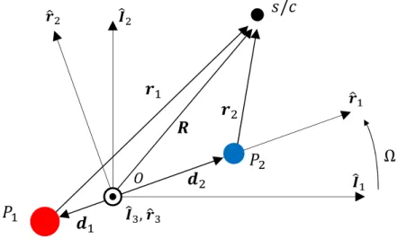
Figure 2.1: Circular restricted three-body system with two reference frames: inertial frame ( ˆI-frame) and rotational frame ( ˆr-frame).

where G is the gravitational constant and r₁ andr₂ are the position vectors of the spacecraft relative to the primaries. The simplified model (2.1) obtained by ignoring the spacecraft mass is called the restricted three-body problem (RTBP). Because the primaries interact only with each other, they orbit around their barycenter. In the special case of the RTBP, we have the circular restricted three-body problem (CRTBP) and the elliptic restricted three-body problem (ERTBP), in which the primaries move in circular and elliptic orbits, respectively.

2.2 Circular Restricted Three-Body Problem

2.2.1 Equation of motion

The CRTBP is a widely used three-body problem for the analysis of spacecraft motion. In this model, two assumptions are made. One is adopted the RTBP: the mass of the spacecraft is negligible. The other is that the primaries move in circular orbits about their barycenter.

Consider two frames as shown in Fig. 2.1: an inertial frame ( ˆI-frame) and a rotating frame ( ˆr-frame). The ˆI-frame is centered at the barycenter O. The ˆr-frame is also centered at the barycenter O; however, the first axis ˆr₁ is aligned with the vector from P₁ to P₂, the third

axis ˆr₃ is normal to the orbital plane of the primaries, and the second axis ˆr₂ completes the right-handed triad.

Because the motion of the primaries is circular, the distance between the primaries d and the angular velocity of the reference frameΩare constant. Thus, all the variables in these frames are normalized such that the following quantities appear as unity: the total mass of the system m₁+m₂, the distance between the primaries d, and the angular frequencyΩ. Note that because the time is also normalized, the variable t in the following discussion is non-dimensional time.

By introducing the mass ratioµ, we can set m₁=1−µ ^{and m}2=µ ^withµ ^<0.5 without loss of generality. LetR=

[

X Y Z

]_T

andΞ=

[ ξ1 ξ2 ξ3

]_T

be the position vectors of the spacecraft in the ˆr-frame and the ˆI-frame, respectively. The relation between them is given by

Ξ=C^I/r(t)R (2.2)

where

C^I/r(t) =







cost −sint 0 sint cost 0

0 0 1





 (2.3)

Differentiating Eq. (2.2) with respect to non-dimensional time yields

Ξ˙ =C˙^I/r(t)R+C^I/r(t)R˙ (2.4)

Ξ¨ =C¨^I/r(t)R+2 ˙C^I/r(t)R˙ +C^I/r(t)R¨ (2.5) The spacecraft position vectors relative to the primaries,r₁andr₂, in the ˆr-frame are given by

r₁=R−d₁ (2.6)

r₂=R−d₂ (2.7)

where d₁ =

[ −µ ^{0 0 ]T, d2 = [ 1}−µ ^{0 0 ]T.} Substituting Eqs. (2.5), (2.6), and

(2.7) into normalized Eq. (2.1) and multiplying the left-handed side by (

C^I/r )₋₁

yields the equations of motion of the spacecraft:

R¨ −KR˙ −KR=−1−µ

|r₁|³ (R−d₁)− µ

|r₂|³(R−d₂) (2.8)

2.2. Circular Restricted Three-Body Problem 15 where

K =







0 2 0

−2 0 0

0 0 0





, K =







1 0 0 0 1 0 0 0 0





 (2.9)

Defining an effective potential function V(R) =1

2

(X²+Y²)

+1−µ

|r₁| + µ

|r₂| (2.10)

transforms Eq. (2.8) into

R¨ −KR˙ =∇V(R) (2.11)

LetX = [

R^T R˙^T ]T

be the state vector. Then, Eq. (2.11) is represented in the first-order form as

X˙ =F(X) (2.12)

with

F(X) =



 R˙

∇V(R) +KR˙



 (2.13)

Equations (2.11) and (2.12) govern the motion of the spacecraft under the gravitational influence of the primaries.

The dot product between Eq. (2.11) and ˙Ryields, in component form, X ¨˙X−2 ˙X ˙Y =X˙∂^V

∂^X Y ¨˙Y+2 ˙Y ˙X =Y˙∂^V

∂Y (2.14)

Z ¨˙Z=Z˙∂^V

∂^Z The addition of these components yields

X ¨˙X+Y ¨˙Y+Z ¨˙Z=X˙∂^V

∂^{X +Y˙}

∂^V

∂^{Y +Z˙}

∂^V

∂^{Z =V˙ (2.15)}

ܮ

ܮ

ܮ

ܮ

ܮ

Figure 2.2: Configuration of Lagrangian points.

Integration of Eq. (2.15) yields the expression for the Jacobi constant, C_Jacobi:

X˙²+Y˙²+Z˙²=2V−C_Jacobi (2.16) This integral of the motion is the only integral of the motion and it is employed in the numerical integration to guarantee the accuracy of the propagated solution.

2.2.2 Libration points

In the CRTBP, five stationary points, which are known as Lagrangian points, can maintain a certain position relative to the two dominant bodies. This is due to the balance of the combined gravitational forces of the primaries and the centrifugal force generated by the rotation of the

ˆ

r-frame. All the Lagrangian points lie in the orbital plane of the primaries. As shown in Fig. 2.2, three of them lie on the straight line connecting the primaries (i.e. ˆr₁-axis) and the other two points each forms an equilateral triangle with the primaries; they are called collinear and triangular equilibrium points, respectively. The three collinear points are unstable whereas the two triangular points are stable. The stability of the Lagrangian points is discussed in

2.2. Circular Restricted Three-Body Problem 17 Appendix A.1.

The Lagrangian points L_i satisfy Eq. (2.11) by eliminating the velocity and acceleration terms:

∇V(R) =0 (2.17)

The Lagrangian points are expressed as

L₁= (l₁(µ^{),0,0), L}2= (l₂(µ^{),0,0), L}3= (l₃(µ^),0,0) L₄= (1/2−µ^{,√3/2,0), L}5= (1/2−µ^,−√

3/2,0) where li(µ⁾are determined by setting Y =0 and solving∂V

∂^{X =}0. To describe the motion near a libration point L_i, it is convenient to use the coordinate system with its origin at L_i(referred to as ˆL_i-frame). Let L_i=

[

lx,i ly,i 0 ]T

andr = [

x y z ]T

be the position vectors of a Lagrangian point and the spacecraft relative to the Lagrangian point, respectively. Replacing Rwithr+L_iand rewriting Eq. (2.11) in the ˆL_i-frame yield

¨

r−Kr˙ =∇U(r) (2.18)

where

U(r) =V(r+L_i) = 1 2 [

(x+l_x,i)²+ (y+l_y,i)² ]

+1−µ

|r₁| + µ

|r₂| (2.19)

r₁=r+L_i−d₁ (2.20)

r₂=r+L_i−d₂ (2.21)

Letx= [

r^T r˙^T ]_T

be the state vector. Then, Eq. (2.18) is represented in the first-order form as

˙

x=f(x) (2.22)

with

f(x) =



 r˙

∇U(r) +Kr˙



 (2.23)

2.2.3 Variational equations

The variational equations are developed for various purposes, including the stability analysis of the Lagrangian points and targeting strategies for the periodic orbits. At an equilibrium point of the system (2.14), the following relations must be satisfied:

∂^V

∂^X

0

= ∂^V

∂^Y

0

= ∂^V

∂^Z

0

=0 (2.24)

where the subscript 0 refers to evaluation at the equilibrium points. Assume a small displacementδ^r=[ ξ η ζ ^]T from the equilibrium point, i.e.

R=L_i+δ^{r (2.25)}

Then, the partial derivative of V with respect to each direction is expanded by the Taylor series at the equilibrium point as follows:

∂^V

∂X(R)≈ξ ∂^2V

∂X²

0

+η ∂^2V

∂X∂Y

0

(2.26)

∂^V

∂^Y(R)≈ξ ∂^2V

∂^X∂^Y

0

+η ∂^2V

∂^Y2

0

(2.27)

∂^V

∂^Z(R)≈ζ ∂^2V

∂^Z2

0

(2.28) where the second-order terms are truncated. Then, Eq. (2.14) becomes

ξ¨−2 ˙η^=VX X^∗ ξ^+VXY^∗ η ^(2.29) η¨ ^{+2 ˙}ξ ^=VXY^∗ ξ^+VYY^∗ η ^(2.30)

ζ¨^=VZZ^∗ ζ ^(2.31)

where the coefficients are V_{X X}^∗ = ∂^2V

∂^X2

0

, V_XY^∗ = ∂^2V

∂^X∂^Y

0

, V_YY^∗ = ∂^2V

∂^Y2

0

,V_ZZ^∗ = ∂^2V

∂^Z2

0

Note that, from Eq. (2.31), the out-of-plane motion is independent of the in-plane motion and is a simple harmonic motion with frequencyω_ζ ^=√|V_ZZ^∗ |. Therefore, the general solution for ζ can be written as

ζ ^=A_ζ^sin(ω_ζ^t+ψ_ζ^{) (2.32)}

2.2. Circular Restricted Three-Body Problem 19 where A_ζ is a constant and ψ_ζ is the phase angle. Since V_ZZ^∗ <0, the eigenvalues of the characteristic equation corresponding to Eq. (2.31) are purely imaginary, which implies that the linear solution is marginally stable. Correspondingly,ξ ^andη are coupled in the in-plane motion. This system can be expressed in first-oder form by defining a state vector δ^xin = [ ξ η ξ^˙ η^{˙ ]Tas}

δ^x˙in =A_inδ^xin (2.33)

with the constant matrixA_in given by

A_in=











0 0 1 0

0 0 0 1

V_{X X}^∗ V_XY^∗ 0 2 V_XY^∗ V_YY^∗ −2 0











(2.34)

The general solutions to this system are

ξ ⁼

∑

i=1

A_ie^λit (2.35)

η⁼

∑

i=1

B_ie^λit (2.36)

where A_i and B_i are constants, but not independent, andλi are the roots of the characteristic equation ofA_in represented by

λ^{4+ (4}−V_{X X}^∗ −V_YY^∗ )λ^2+(VX X^∗ V_YY^∗ −V_XY^{∗ 2} )

=0 (2.37)

For any eigenvalue, the quantities Aiand Biare scalar multiples. Therefore Bi=αiAi, which is confirmed by differentiating Eqs. (2.35) and (2.36) and substitution into Eqs. (A.1) and (A.2).

Considering the collinear Lagrangian points, the characteristic equation (A.10) has two real eigenvalues (λ1,λ2 = −λ1) and two imaginary eigenvalues (λ3, λ4 =−λ3). At least one eigenvalue includes a positive real part; thus, Li(i=1,2,3) are unstable. In general, ξ ^and η become unbounded trajectories as t → ∞. However, by selecting initial conditions that

eliminate the divergent mode, the solutions to Eqs. (2.35) and (2.36) are simplified to the isolate oscillators as

ξ ^=A3e^λ3t+A₄e^−λ3t (2.38)

η ⁼α3

(

A₃e^λ3t−A₄e^−λ3t )

(2.39) The coefficients A₁ and A₂ corresponding to the real eigenvalues are chosen to be zero. The set of Eqs. (2.38), (2.39), and (2.36) provides a good initial guess for a small periodic or quasi-periodic orbit in the vicinity of the Lagrangian points.

2.2.4 Periodic orbits

Periodic solutions exist in the vicinity of a collinear Lagrangian point in the CRTBP.

From the analysis in the previous subsection, the linearized dynamics around the collinear libration points is that of the product of a saddle (two real opposite eigenvalues) and a four-dimensional center (two pairs of imaginary eigenvalues) [96]. Thus, giving an appropriate initial condition only in the direction of the center branch provides periodic orbits [97].

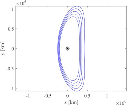
The planar orbits and three-dimensional orbits are called Lyapunov orbits and halo orbits, respectively. Figures 2.3 and 2.4 show five different Lyapunov orbits and ten different halo orbits around the Sun-Earth L₁ point in the ˆL₁-frame, respectively. Owing to the z-axis symmetry of the CRTBP dynamics, two types halo orbits exist: northern halo orbits and southern halo orbits.

Because the CRTBP does not have any analytic solution, periodic or quasi-periodic orbits are difficult to obtain. The problem is highly nonlinear and small variations in the initial conditions break the periodicity of the orbit. As an analytical approach, Richardson constructed first- and third-order approximations by linearizing the equations of motion, which facilitates the generation of periodic orbits with desired amplitudes [41]. On the other hand, Howell developed a numerical approach based on the state transition matrix and the mirror theorem [98], which produces highly nonlinear periodic orbits.

2.2. Circular Restricted Three-Body Problem 21

-1 -0.5 0 0.5 1

x [km] ₁₀⁶

-1 -0.5 0 0.5 1

y [km]

10⁶

Figure 2.3: Lyapunov orbits around Sun-Earth L₁point: the symbol∗denotes L₁Lagrangian point.

2.2.5 Invariant manifolds

In the CRTBP, there are stable and unstable manifolds known as invariant manifolds.

These manifolds are associated with the Lagrangian points (denoted by W_Li) or periodic orbits (denoted by WPO). The former manifolds WL_i can be obtained directly from the eigenvalues and the corresponding eigenvectors of the Jacobian matrix of this regime. By contrast, the latter manifolds W_PO require the monodromy matrix associated with the orbit to be computed and they can then be obtained from the eigenvectors of the matrix.

Invariant manifolds associated with the equilibrium points

Collinear Lagrangian points are located at the saddle point and possess stable eigenvalues λs and unstable eigenvalues λu. This means that the invariant manifolds associated with the points are two one-dimensional lines. Let x_Li be a state of a saddle-type libration point in the ˆL_i-frame, and let x(t;x₀) be a solution to the system given by Eq. (2.22) for the initial conditionx₀. P(β⁾is defined as a neighborhood of β^{, where} β denotes a state or an orbit.

5

y [km]

10⁵ 0

-6 -5 -4 -2

10⁵

x [km]

0 10⁵

z [km]

2 4

0 6

2 4

Figure 2.4: Halo orbits around Sun-Earth L₁ point: the blue and red orbits denotes northern and southern halo orbits, respectively; the symbol∗denotes the L₁Lagrangian point.

The stable and unstable manifolds associated with the libration point (denoted by W_L^s

i and W_L^u

i, respectively) are given by

W_L^s_i={x₀∈P(x_Li)|lim

t→∞x(t;x₀) =x_Li=0} (2.40) W_L^u_i={x₀∈P(xL_i)| lim

t→−∞x(t;x₀) =xL_i =0} (2.41) These invariant manifolds are curves that originate from the libration point, as shown in Fig.2.5.

The linearized dynamics of Eq. (2.22) is

˙ x= ∂^f

∂^x

0

x≜Ax (2.42)

where the matrix A is the Jacobian matrix. This matrix has six eigenvalues: two pairs of purely imaginary numbers and one pair of real numbers. Let vs and vu be the eigenvectors corresponding to the stable and unstable eigenvalues, respectively. The invariant manifolds are

2.2. Circular Restricted Three-Body Problem 23

-2 -1 0 1 2

x [km] ₁₀⁶

-2 -1.5 -1 -0.5 0 0.5 1 1.5 2

y [km]

10⁶

Earth

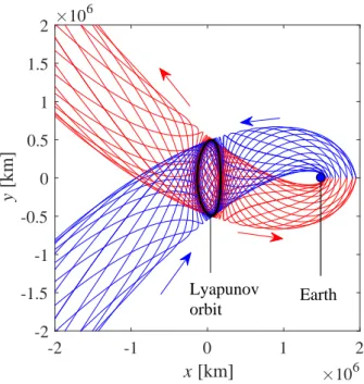
Figure 2.5: Invariant manifolds associated with the Sun-Earth L₁ point: the symbol ∗ is denotes L₁Lagrangian point; the blue and red lines denote the stable and unstable manifolds, respectively.

easily obtained from the propagation of the perturbed state from the point in the direction of the stable and unstable eigenvectors. The stable manifold W_L^s

i can be obtained by backward propagating the following state in time:

x^s_Li =x_Li±ε ^vs

|v^s| (2.43)

whereεis the size of the perturbation from the points. Similarly, the unstable manifold W_L^u_ican be computed by forward integrating the initial state:

x^u_Li=xL_i±ε_|^vu

v^u| (2.44)

Note that the signs± of the perturbation yield two parts of each manifold; one will generate the motion that departs the point towards the secondary body, and the other will generate the motion that departs the point away from the secondary body.