39
Grouping health and related indicators in Japan: similarities between hierarchical cluster analysis and principal component analysis
MMH Khan, Mitsuru M ORI
Department of Public Health, Sapporo Medical University School of Medicine, South 1, West 17, Chuo-ku, Sapporo 060-8556, Japan
(Chief: Prof. M. Mori)
ABSTRACT
Japan yearly publishes several health and related indicators by 47 prefectures, which could be presented by a fewer number of groups using both hierarchical cluster analysis (HCA) and principal component analysis (PCA). As no study involving both HCA and PCA, applied to the data set of heath indicators, was found in Japan, our study pur- poses were: (i) to determine fewer groups of indicators from the 40 health and related indicators by applying both methods, and then (ii) to compare their groups with each other. First HCA was applied to the data to have the dendro- gram of 40 indicators, after that the dendrogram was analyzed by dendrogram sharpening technique to identify the smaller groups (clusters) of either 1 or 2 indicators for the exclusion purpose from further analysis. Remaining 30 indicators (after dropping 10 indicators by dendrogram sharpening) were regrouped by HCA and compared with the groups of PCA. Reanalyzing them, HCA identified five groups (clusters) which were labeled as C1: health care facil- ity and cause-specific mortality , C2: morbidity , C3: welfare opportunity , C4: overall mortality , and C5:
social status . Similarly PCA showed 5 groups (PCs) which explained 86% of the total variation. These were labeled as P1: health care facility , P2: socio-economic standard and cause-specific mortality , P3: welfare opportunity , P4: morbidity , and P5: overall mortality . Comparative results revealed C2=P4, C3=P3, and C4=P5, whereas remaining groups overlapped highly by indicators. This study revealed that after dendrogram sharpening, both HCA and PCA provided almost similar groups of indicators and hence indicated their applicability to the same set of data.
Dendrogram sharpening also made the interpretation more understandable by dropping the smaller groups of indica- tors.
(Received August 9, 2004 and accepted October 6, 2004) Key words: Health indicators, Grouping, Dendrogram, Japan
1 Introduction
Considerably numerous applications of multivariate cluster analysis (CA)
1-11)as well as factor analysis (FA)
12-26), that usually take a larger number of indicators (also referred as objects/variables) and then reduce them to a smaller number of groups (also referred as clusters or principal components-PCs) based on their similarities
27-29), have indicated their importance in many fields such as agriculture, anthropology, biology, chemistry, climatol- ogy, demography, ecology, economics, food research, genetics, geology, medical research, meteorology, nurs- ing, oceanography, psychology, quality control, sociolo- gy, and so on
27,28,30,31). Although most of the available stud- ies applied only one of the above-mentioned two multi- variate techniques for analyzing the data, there are some studies where both of these techniques were applied to
the same set of data mainly for comparing/validating their findings with each other
32-36).
In fact Japan regularly (yearly basis) publishes sev- eral indicators for indicating the overall socioeconomic, demographic, health and medical conditions of the coun- try. For example, crude mortality rate, infant mortality rate, neo-natal mortality rate, post neo-natal mortality rate, under five mortality rate, perinatal mortality rate, age-adjusted mortality rate, still birth rate, life-expectancy at birth or any particular age such as 20, 40, 60, and so on are published to indicate the mortality situation of the country. Similarly for indicating medical and health care conditions, many indicators are available which may be based on medical doctors, nurses, hospitals, clinics, hos- pital utilization, bed utilization in hospitals and clinics, disability, medical attendance, medical symptoms, cause
ORIGINAL
specific mortality related to both communicable and non- communicable diseases, and so on. Because of similari- ties in the interpretation of some indicators, it may be desirable for the researchers not to use all the indicators separately but to make significantly smaller number of groups based on their homogeneity that the objects within the same group share. Both CA and FA are the ways to reduce a large number of indicators into a smaller number of dimensions (groups) that are comprehensible
33)and hence provide researchers the opportunity to interpret their findings in an understandable way. Although several methods are available for doing CA and FA
27,29), applica- tions of the method of hierarchical cluster analysis (HCA) from CA or principal component analysis (PCA) from FA are more frequent than others.
Although Japan has been publishing regularly sever- al updated indicators by 47 prefectures, to our knowledge there is no study which applied both methods (HCA and PCA) to the same data set of Japanese health and related indicators. Therefore the study purposes were: (i) to determine fewer groups of indicators by both methods by analyzing the health and related indicators which are yearly published in Japan by two sources
37,38), and then (ii) to compare the groups of HCA with the groups of PCA.
Initially HCA (between-groups/average linkage method) was applied to the whole set of data to make the dendro- gram, and then the dendrogram sharpening technique, as explained by Stanberry et al
2)., was carried out to drop smaller clusters of size either 1 or 2 indicators (may be outliers) from further analysis. The remaining indicators after dendrogram sharpening were reanalyzed by HCA to have the revised dendrogram and finally the groups of HCA derived from dendrogram were compared with the groups of PCA (varimax/orthogonal rotation method).
Hopefully comparative findings of these techniques would provide some useful information about the group- ings of indicators and their applicability to the same set of data. The comparative findings as well as the ordering of groups may also indicate the importance of the PCs in PCA and closeness of the clusters in HCA.
2 Methods
2.1 Selection of health and related indicators
The study used the recent data of 40 indicators (Table 1) which are regularly published for 47 prefectures in Japan by the two well-known sources
37, 38). These sources are widely available as well as reliable in Japan.
We selected most of the important indicators from these sources for analytical purpose, which mainly covered the
statistics of mortality rate (crude, age-adjusted, infant, neonatal, and perinatal), cause-specific mortality rate (heart disease, malignancy, stroke, and suicide), fertility rate (birth rate, and still birth rate), disability rate (propor- tion of disability in life, and proportion of any symptom of health condition e.g., back pain), utilization rate of medical facilities (proportion of hospitalization in a day, proportion of medical attendance, and proportion of receiving outpatient medical services), availability of medical facilities (doctors, hospitals, medical beds in hos- pitals, and medical beds in clinics), marital status (marital rate, and divorce rate), life expectancy, socio-economic status (rate of population who need social support, yearly income, yearly medical expenditure, percent of admission into college/university, percent of population having own house). As the data for different indicators were not available for any single year, we used data from 1999 to 2002 depending on availability of them. Some indicators were chosen for both male and female separately again depending on the availability of them.
2.2 Statistical techniques
This study used SPSS 10.0 to carry out the analysis.
The detailed of the SPSS analysis including the descrip- tion of HCA and PCA were found elsewhere
27-29). However, a brief description about them is given below:
2.2.1 Hierarchical cluster analysis
Hierarchical clustering begins by finding the closest pair of objects according to distance (similarity) measure and combines them to form a cluster. The algorithm con- tinues one step at a time, joining pairs of objects, pairs of clusters, or an object with a cluster, until all the data are in one cluster. Average linkage method simply joins the variables or clusters on the basis of the least distance (most similarity) between them at each successive stage of the analysis. Pearson's correlation co-efficient is used as similarity measure. Two variables showing strongest correlation coefficient are grouped at the first stage. At the second stage, two variables or clusters showing sec- ond strongest correlation coefficient are joined, and so on.
The resulting clusters can be presented graphically by the
dendrogram (Fig. 1 and Fig. 2). The pairs of indicators in
the same cluster are more similar than the pairs of clusters
that are placed into other clusters. The agglomeration
schedule (not shown) can be used to show the clustering
stages with similarity measures.
2.2.2 Dendrogram sharpening
According to Stanberry et al
2)the goal of dendro- gram sharpening technique is to reduce the number of considered objects, by deleting or agglomerating them, and at the same time by preserving as much structure of the data as possible. In practice, in a large data set the observations in the tails contaminate the picture (dendro- gram), filling the space between the modal peaks. The
known solution to this problem is to alter the original col- lection of objects in order to reveal its underlying struc- ture. One natural alternation is to sharpen the data to increase the contrast between the density regions.
Although there are several ways to perform the dendro- gram sharpening, our study exactly followed Stanberry et al
2). As different terminologies such as root node, node, parent node, terminal node, left child, right child, size of Table1 Selected indicators with mean and standard deviation (S.D.)
Description of selected indicators Mean S.D.
1 Age adjusted total mortality rate, female (2000
*) 320.1 15.1
2 Age adjusted total mortality rate, male (2000
*) 635.9 32.3
3 Crude birth rate (2001
†) 9.3 0.8
4 No. of clinics, both-sexes (2001
*) 74.2 12.7
5 Crude mortality rate, (2001
†) 8.4 1.1
6 Divorce rate, both-sexes (2001
*) 2.2 0.3
7 No. of hospitals, both-sexes (2001
*) 8.5 3.3
8 Infant mortality rate, birth (2001
†) 3.2 0.6
9 Life expectancy, female (2000) 84.7 0.4
10 Life expectancy, male (2000) 77.6 0.6
11 Marital rate, both-sexes (2001
†) 5.9 0.6
12 Medical beds in clinics, both-sexes (2001
*) 224.3 136.0
13 Medical beds in hospitals, both-sexes (2001
*) 1439.0 361.5
14 Medical doctors, both-sexes (2000
*) 205.9 36.5
15 Mortality from heart diseases, both-sexes (2001
*) 128.1 18.2
16 Mortality from cancers, both-sexes (2001
*) 252.3 29.3
17 Mortality from strokes, both-sexes (2001
*) 117.2 25.0
18 Neonatal mortality rate, birth (2001
†) 1.7 0.4
19 Perinatal mortality rate, delivery (2001
†) 5.5 0.6
20 Having disability in life, female (2001
†) 115.6 10.7
21 Having disability in life, male (2001
†) 96.0 10.8
22 Hospitalization rate in a day survey, female (2001
*) 1361.7 430.7
23 Hospitalization rate in a day survey, male (2001
*) 1266.6 356.7
24 Medical attendance, female (2001
†) 334.2 23.3
25 Medical attendance, male (2001
†) 286.9 20.4
26 Recipient of medical services in a day of survey, female (1999
*) 7443.3 1084.5
27 Recipient of medical services in a day of survey, male (1999
*) 6127.6 951.8
28 Recipient of outpatient medical services in a day of survey, female (1999
*) 6081.2 770.0 29 Recipient of outpatient medical services in a day of survey, male (1999
*) 4862.4 669.2
30 Having any medical symptoms, female (2001
†) 356.5 21.4
31 Having any medical symptoms, male (2001
†) 283.6 19.1
32 Still birth rate, delivery (2001
†) 31.8 5.5
33 Suicide rate, both-sexes (2001
*) 24.0 4.1
34 Rate of people who need social support, both-sexes (2000
†) 7.2 4.2
35 Yearly income ( 000 Japanese Yen) per person (2000) 2849.1 373.4
36 Proportion of job seekers who found a job (2002) 0.5 0.1
37 % of people having own house (2000) 66.8 7.2
38 % of female admission into college/university (2002) 41.2 6.5
39 % of male admission into college/university (2002) 45.4 6.9
40 Yearly medical expenditure per person (1999) 256.7 36.1
Source : Health and Welfare Statistics Association
37)and Asahi Newspaper Co. Ed.
38)*
: rate expressed as 100,000,
†: rate expressed as 1,000. Year of data is indicated in parenthesis
the agglomerated cluster, n
fluff, n
core, are clearly explained by Stanberry et al
2), we did not explain them here.
Following the paper of Stanberry et al
2)., where the sharp-
ening process was controlled by only two parameters: n
fluff≤ 2 and n
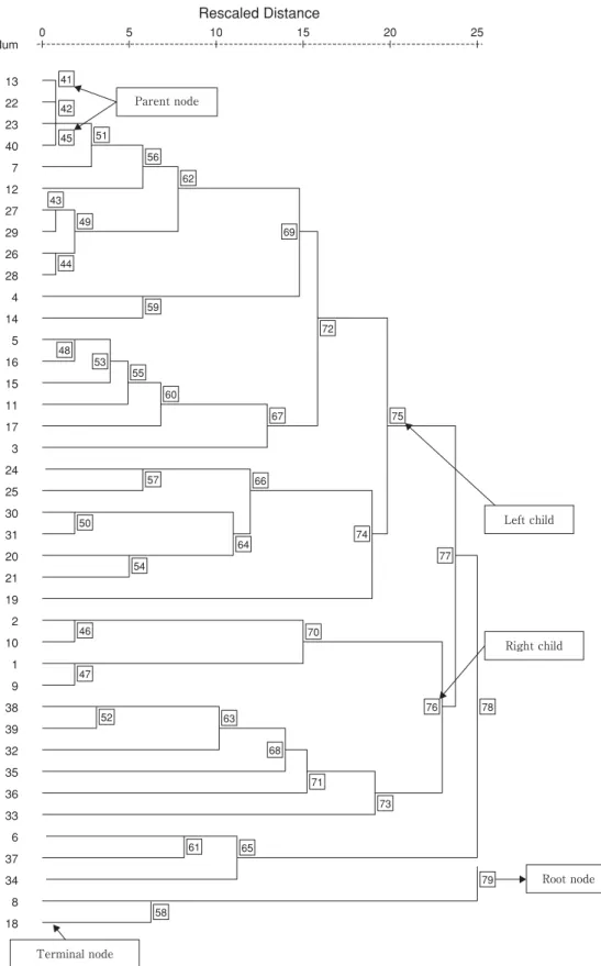
core>5, our study started the sharpening process from the root node of the tree 79, where all nodes were
0 Num
Rescaled Distance
13 22 23 40 7 12 27 29 26 28 4 14 5 16 15 11 17 3 24 25 30 31 20 21 19 2 10 1 9 38 39 32 35 36 33 6 37 34 8 18
5 10 15 20 25
41 42 45 51
56 62
69
72
67 75
74
70
76 78
79 77 43
49
44
59
48 53
55
57
50
54
46
47
52 63
68 71
73
61
58
65 64
66 60
Parent node
Left child
Right child
Root node
Terminal node
Fig. 1 Dendrogram using average linkage (between groups) method for 40 objects
indicated by number given in the squared boxes (Fig. 1).
The size of the root node was equal to the number of the terminal nodes (i.e. 40 terminal nodes). Since the size 40 was greater than 5, the root node was subject to sharpen- ing. It had two children: the left child 78 had a size of 38 and the right child 58 had a size of 2. Hereafter the size of the node will be indicated as a number in parenthesis.
Node 58 was discarded because the size of node was ≤ 2 which satisfied the original condition. The size of the left child 78 (38) was greater than 2, so it remained unchanged. Then the left child 77 (35) and right child 65 (3) of the node 78 were analyzed again. Both of them remained unaltered because they were of size greater than 2. Since the size of the node 77 (35) was greater than 5, the left child 75 (25) and right child 76 (10) of node 77 were analyzed next. Both children were subject to sharp- ening because the size for each of them was greater than 5. The left child 70 (4) of the node 76 remained unchanged since the size was less than 5 but greater than 2. However, the right child 73 (6) of the node 76 was sharpened again and the right single point child was dis- carded. Left child 71 (5) of the node 76 remained unchanged. The same process of sharpening was contin- ued until it was required by the given conditions.
2.2.3 Principal component analysis
PCA has gained increasing acceptance and populari- ty over the past 30 to 40 years. It is probably the oldest and best known among the multivariate techniques. The central idea of it is to reduce the dimensionality of a set of data consisting of a large number of interrelated variables, while retaining as much as possible of the variation pres- ent in the data set. This reduction is achieved by trans- forming to a new set of variables (also called principal components (PCs)), which are uncorrelated and which are ordered so that first few retain most of the variation pres- ent in all of the original variables. Each extracted PC has an eigenvalue which shows the proportion of variance accounted for by each PC (not each variable). Varimax rotation was used to achieve what is called simple struc- ture, that is, high factor loadings on one of the PCs and low loadings on all others. Factor loadings vary between -1 to +1 and indicate the strength of relationship between a particular variable and a particular PC, in a way similar to a correlation. In an ideal world, each of the original variables will load highly (e.g., >0.5) on one of the PCs and low (e.g. <0.2) on all others. However, there may be some irritating variables that end up with loading on the wrong PC and show high loading on several PCs.
2.2.4 Comparison of two methods
CA analysis of variables resembles FA because both procedures identify related groups of variables. Both CA and FA have a number of options to find the underlying clusters (in CA) and factors (in FA) of variables.
Although there are some similarities between two meth- ods, they differ in several important ways. Such discrep- ancies can occur because of differences in how the two approaches handle the relationships between items.
Among the discrepancies, the following may be notable:
(i) FA particularly PCA has an underlying theoretical model, while cluster analysis is more ad hoc. PCs can be found using purely mathematical arguments; they are given by an orthogonal linear transformation of a set of variables optimizing a certain algebraic criterion.
Mathematically, FA is similar to a forward run in multiple regression analysis. (ii) CA is hierarchical, and it is driv- en by the strength of individual correlations; in contrast, FA considers the relationships between all variables simultaneously. (iii) FA is used to reduce a larger number of variables to a smaller number of factors that describe these variables, whereas CA is more frequently used to group the cases rather than variables that shared similar features with each other, (iv) FA analyzes all variables at each factor extraction step to calculate the variance that each variable contributes to that factor, whereas CA cal- culates similarity or distance between each variable/case and every other variable/case and then it groups the two variables/cases that have the greatest similarity or the least distance in a cluster of two. (v) Although ad hoc, PCA has some rules-of-thumb to select the number of PCs, while CA does not have any such rule
27-29).
3 Results
HCA was applied to the data before and after den- drogram sharpening. Before dendrogram sharpening, we included all the 40 variables to have a dendrogram (Fig.
1). This figure showed some clusters with one or two ter-
minal nodes or original variables. For example, suicide
rate (terminal node) only made a sub-cluster in the den-
drogram. To avoid such small clusters we used sharpen-
ing method using above-mentioned criteria and dropped
10 original variables such as suicide rate, birth rate, peri-
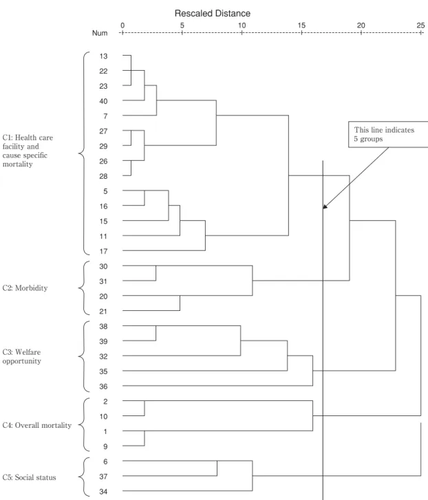
natal mortality rate, and so on for further analysis. Fig. 2
presented the dendrogram of 30 objects after sharpening
which showed five groups (clusters) of variables (indicat-
ed by a straight line superimposed on the Fig. 2). Each
cluster was referred by a name. These names of the clus-
ters were C1: health care facility and cause specific
mortality , C2: morbidity , C3: welfare opportuni- ty , C4: overall mortality , and C5: social status . The given names were based on the variables which they included. For example, second cluster was labeled as C2: morbidity because it included 4 variables relating to having any medical symptoms (e.g back pain) and hav- ing disability symptoms in the life.
Similarly analyzing 30 objects PCA extracted 5 dis- tinct groups (PCs) (Table 2), labeled as P1: health care facility , P2: socio-economic standard and cause-spe- cific mortality , P3: welfare opportunity , P4: mor- bidity , and P5: overall mortality respectively, on
the basis of factor loading found after varimax rotation (eigenvalue >1.0). The rotation converged in 8 iterations and the rotated eigenvalues of the five PCs were 8.90, 5.16, 4.25, 4.17, and 3.39 respectively. These PCs explained 86% of the total variance, accounting for 29.70%, 17.20%, 14.17%, 13.91%, and 11.29% respec- tively. The 1
stPC was labeled as P1: health care facili- ty since it included 9 variables that were related to health and medical care facilities and explained the great- est variance among the variables. According to the infor- mation, P1: health care facility was greatly loaded on some variables like hospitalization rate, medical beds in
0 Num
13 22 23 40 7 27 29 26 28 5 16 15 11 17 30 31 20 21 38 39 32 35 36 2 10 1 9 6 37 34
5 10 15 20 25
C1: Health care facility and cause specific mortality
C2: Morbidity
C3: Welfare opportunity
C4: Overall mortality
C5: Social status
This line indicates 5 groups
Rescaled Distance
Fig. 2 Revised dendrogram for 30 objects using average linkage method after dendrogram sharpening
hospitals and number of hospitals and so on. The 4
thPC P4: morbidity was highly loaded on the variables relat- ed medical symptoms and disability. Similarly the 5
thPC P5: overall mortality was inversely loaded on life expectancy but positively loaded on age adjusted total mortality.
Comparison of five groups presented in Table 2 (made by PCA) and Figure 2 (made by HCA) revealed that both PCA and HCA methods provided almost similar groupings of indicators although they are different by the above-mentioned points given in methods. For instance, three groups of HCA namely C2: morbidity , C3:
Table2 Principal factor loading matrix for 5 PCs (using the variables remained after dendrogram sharpening)
Var. Principal components and indicators Principal components (PCs)
No. 1 2 3 4 5
P1: Health care facility
7 No. of hospitals
0.95- - - -
22 Hospitalization rate in a day of survey, female
0.94- -0.23 0.10 -
13 Medical beds in hospitals
0.94- -0.23 0.10 -
23 Hospitalization rate in a day of survey, male
0.920.12 -0.31 0.12 -
40 Yearly medical expenditure per person
0.910.12 -0.20 0.31 -
27 Recipient of medical services in a day of survey, male
0.820.19 -0.16 0.43 0.16 26 Recipient of medical services in a day of survey, female
0.790.13 -0.19 0.41 0.20 29 Recipient of outpatient medical services in a day of survey, male
0.680.21 - 0.55 0.25 28 Recipient of outpatient medical services in a day of survey, female
0.590.17 -0.14 0.52 0.33
P2: Socio-economic standard and cause-specific mortality
37 % of people having own house -
0.89- - -
17 Mortality from strokes 0.28
0.83-0.20 - 0.13
6 Divorce rate 0.20
-0.82-0.19 -0.13 0.24
15 Mortality from heart diseases 0.50
0.75- 0.18 0.19
5 Crude mortality rate 0.55
0.74-0.18 0.22 0.12
11 Marital rate -0.47
-0.720.32 -0.22 -
16 Mortality from cancers 0.49
0.63-0.22 0.41 0.24
34 Rate of people who need social supports 0.46
-0.57-0.39 - 0.29
P3: Welfare opportunity
39 % of male admission into college/university -0.25 -0.18
0.850.26 -
38 % of female admission into college/university -0.12 -0.20
-0.820.27 -
36 Proportion of job seekers who found a job -0.10 0.25
0.79- -0.17
32 Still birth rate 0.52 -0.14
-0.64-0.15 -
35 Yearly income per person -0.44 -0.33
0.63- 0.14
P4: Morbidity
30 Having any medical symptoms, female 0.11 - 0.29
0.91-
31 Having any medical symptoms, male 0.12 - 0.31
0.86-
20 Having disability in life, female 0.32 0.33 -
0.79-0.12
21 Having disability in life, male 0.50 0.29 -
-0.66-
P5: Overall mortality
9 Life expectancy, female 0.20 - - -
-0.941 Age adjusted total mortality rate, female - -0.15 - -
0.922 Age adjusted total mortality rate, male 0.24 - -0.47 -
0.7510 Life expectancy, male -0.35 -0.12 0.50 -
-0.70Rotated eigenvalue: 8.91, 5.16, 4.25, 4.17, and 3.39
% of total variance explained (rotated): 29.68, 17.20, 14.17, 13.91, and 11.29
Cumulative % of total variance explained: 29.68, 46.88, 61.05, 74.97, and 86.25
Note : Rotation converged in 8 iterations. - : indicated loading was <0.10.
welfare opportunity , and C4: overall mortality were completely similar (except order) to the three groups of PCA namely P4: morbidity , P3: welfare oppor- tunity , and P5: overall mortality respectively.
Indicators of other two groups such as C1: health care facility and cause specific mortality , and C5: social class made by HCA and P1: health care facility and P2: socio-economic standard and cause specific mortality made by PCA overlapped remarkably.
4 Discussion
The findings of the present study signified the impor- tance of using HCA and PCA for analyzing and interpret- ing a large number of quantifiable health and related indi- cators by a fewer number of groups meaningfully. This study illustrated how to avoid small-size clusters (may be outliers) by dendrogram sharpening technique. Detecting outliers to remove or diminish their effects was desirable because these may have a drastic and disproportionate influence on the results of various analyses of a data set
28). The analysis of 30 indicators (which remained after den- drogram sharpening) by both HCA and PCA demonstrat- ed that health and related indicators could be grouped into 5 distinct groups in case of Japanese context. The findings clearly indicated that there were many indicators that tend- ed to cluster under some underlying groups. For example, 9 different indicators of the 1
stPC P1: health care facili- ty tended to show their similarities with each other.
Another important finding of the study was to obtain almost similar number of groups of indicators by both techniques. The indicators of the 3 PCs of PCA labeled as P3: welfare opportunity , P4: morbidity , and P5:
overall mortality were completely similar (except order- ing of groups) to the indicators of three clusters of HCA named as C3, C2, and C4 respectively. Two other PCs entitled as P1: health care facility and P2: socio- economic standard and cause-specific mortality consti- tuted remaining two clusters C1 and C5, with noticeable overlapping of the indicators. For example, the 9 indica- tors of the PC P1: health care facility by PCA revealed as a subset of 14 indicators of one cluster C1:
health care facility and cause specific mortality by HCA. Similarly, 3 indicators of the 5
thcluster C5: social status of HCA corresponded as a subset of 2
ndPC P2:
socio-economic standard and cause-specific mortality of PCA.
Although comparative findings of PCA and HCA showed almost similar groupings of indicators, their ordered based on the results were not same. Ordering of
the groups and their interpretation may be important to discuss briefly. For example, the order of the PCs abbre- viated as P1, P2, P3, P4, and P5 in PCA were determined on the basis of rotated eigenvalues (highest to lowest) and total variance explained. In contrast, the order of the clusters abbreviated as C1, C2, C3, C4, and C5 in HCA were determined on the basis of distance measure (i.e., correlation co-efficient). Statistically P1 was most impor- tant than other PCs because it explained greatest amount of total variance. In HCA, the distance was smallest (i.e.
correlation was strongest) between C1 and C2 and hence these two clusters were closest. Similarly the distance was largest (i.e. correlation was smallest) between C1 and C5 and hence these two were least close as compared to other combinations of C1. These discrepancies may be attributed to the methodological differences of two meth- ods.
Rotation was used to interpret the PCs simply and understandably and to avoid intermediate loadings by making larger loadings larger and smaller loading smaller than their unrotated values. However, using loadings to interpret PCs can be misleading without examining corre- lation between variables and PCs
27-29). Although HCA and PCA could be applied in a variety of situations, they are not free from criticisms. In PCA some indicators may act as irritating variables and show higher loadings on two or more PCs
27). For instance, in our study mortality from heart disease, cancers, crude mortality rate, and marital rate showed higher loadings on P2 and P1. Similarly, still birth rate and yearly income per person showed higher loadings on P3 and P1. One of the limitations of the clus- ter analysis was that the results were highly dependent upon the chosen method and the variables used to form the clusters
1). When sets of original points (indicators) become close or overlap, the average linkage algorithm yields several large clusters, giving an impression of dis- tinct grouping in the data regardless of the density. Thus this algorithm is unable to properly indicate the modal peaks unless the data is constituted of well-separated groups of objects
2). The main idea of their algorithm was to discard all small-sized children nodes with a large- sized parent node in the dendrogram. Although the den- drogram sharpening algorithm has many advantages such as (i) it does not require any prior knowledge of the num- ber of clusters or their locations, (ii) it discards the objects which are outliers and provide meaningful results, and (iii) final classification algorithms are both very simple and easy to implement, it has also some disadvantages.
The serious disadvantage of the sharpening is that when
the original data (variables) consist of groups of different densities, there is a great risk that the smallest clusters will be completely removed. Another limitation is the proper specification of the two required sharpening parameters n
fluffand n
core. However, the choice of these values is defined by the size and structure of data set
2). Naming the groups are not always suitable, because the different concepts may be involved in some factors
19).
Using the results of dendrogram (Fig. 1 and Fig. 2) and factor loadings (Table 2), an attempt had been made to discuss the relationship of life expectancy with other indicators. It should be noted that during the last four decades, global average life expectancy at birth increased dramatically from about 50 to 66 years
39). Fortunately, Japan has achieved the highest life expectancy in the world. Changes in several factors such as mortality
39)or standardized mortality ratio
40), fertility
39), education
41)or illiteracy
42), income
41,43)or income inequality
42), gross domestic product
42), marital status and employment sta- tus
41)may be associated with the changes in life expectan- cy. Other factors such as medical interventions
39), reduc- tion/elimination in: (i) cardiovascular and circulatory dis- eases
44), (ii) infant deaths from respiratory diseases
44), (iii) fatal diseases
45), and (iv) cerebrovascular diseases and mortality from stomach cancer
46)may also improve the life expectancy. According to our study among all the indicators age-adjusted total mortality maintained the strongest association with life expectancy as compared to others. The indicators of other groups revealed weaker relationship with life expectancy. Perhaps for this reason, life expectancy is widely used by the health professionals and general public as an indicator for summarizing mor- tality experience of a population
40).
In conclusion, both HCA and PCA are very useful explorative multivariate techniques for grouping the large number of health and related indicators by a significantly fewer number of latent groups. Both statistical tech- niques revealed almost similar groups of indicators, which may indicate their applicability into the same set of data and validate the results of each other. Moreover, induction of dendrogram sharpening technique as well as its usefulness revealed by our study may attract further researches because it showed the way to discard smaller size clusters of either 1 or 2 indicators from a large data set. We recommend the application of sharpening tech- nique, particularly when the researchers will have a large set of indicators, to obtain a clearer representation of the data structure.
References
1. Bischof G, Rumpf HJ, Hapke U, Meyer C, John U. Types of natural recovery from alcohol dependence: a cluster analysis approach. Addiction 2003; 98: 1737-1746.
2. Stanberry L, Nandy R, Cordes D. Cluster analysis of fMRI data using dendrogram sharpening. Hum Brain Mapp 2003;
20: 201-219.
3. Kinoshita S, Takahashi H, Okada M, Nishikawa H, Toyokawa S, Kano K. Geographical pattern of malignant neoplasm by cluster analysis using standardized mortality ratios (SMRs) in Ibaraki, Japan. J Epidemiol 2002; 12: 143- 152.
4. Quatromoni PA, Copenhafer DL, Demissie S, D'Agostino RB, O'Horo CE, Nam B-H, Millen BE. The internal validity of a dietary pattern analysis. The Framingham Nutrition Studies. J Epidemiol Community Health 2002; 56: 381-388.
5. Koo E, Nagy Z, Sesztak M, Ujfalussy I, Meretey K, Bohm U, Forgacs S, Szilagyi M, Czirjak L, Farkas V. Subsets in psoriatic arthritis formed by cluster analysis. Clin Rheumatol 2001; 20: 36-43.
6. Pryer JA, Nichols R, Elliott P, Thakrar B, Brunner E, Marmot M. Dietary patterns among a national random sam- ple of British adults. J Epidemiol Community Health 2001;
55: 29-37.
7. Furmark T, Tillfors M, Stattin H, Ekselius L, Fredrikson M.
Social phobia subtypes in the general population revealed by cluster analysis. Psychol Med 2000; 30: 1335-1344.
8. Kishi S. Characteristics of proportional analysis for soft tis- sue facial profile: epidemiological possibilities of measure- ment item reduction. J Oral Sci 1999; 41: 111-115.
9. Nakao K, Takaishi J, Tatsuta K, Katayama H, Iwase M, Yorifuji K, Shinosaki K, Takeda M. A profile analysis of personality disorders: beyond multiple diagnoses. Psychiatry Clin Neurosci 1999; 53: 373-380.
10. Wu JD, Milton DK, Hammond SK, Spear RC. Hierarchical cluster analysis applied to workers' exposures in fiberglass insulation manufacturing. Ann Occup Hyg 1999; 43: 43-55.
11. Hulshof KF, Wedel M, Lowik MR, Kok FG, Kistemaker C, Hermus RJ, ten Hoor F, Ockhuizen T. Clustering of dietary variables and other lifestyle factors (Dutch Nutritional Surveillance System). J Epidemiol Community Health 2002;
46: 417-424.
12. Masaki M, Sugimori H, Nakamura K, Tadera M. Dietary patterns and stomach cancer among middle-aged male workers in Tokyo. Asian Pac J Cancer Prev 2003; 4: 61-66.
13. Cavallini MC, Bella DD, Siliprandi F, Malchiodi F, Bellodi L. Exploratory factor analysis of obsessive-compulsive patients and association with 5-HTTLPR polymorphism.
Am J Med Genet 2002; 114: 347-353.
14. Hanley AJG, Karter AJ, Festa A, D'Agostino Jr R, Wagenknecht LE, Savage P, Tracy RP, Saad MF, Haffner S.
Factor analysis of metabolic syndrome using directly meas- ured insulin sensitivity: the insulin resistance atherosclerosis study. Diabetes 2002; 51: 2642-2647.
15. Jason LA, Taylor RR, Kennedy C, Jordan K, Huang C-F, Torres-Harding S, Song S, Johnson D. A factor analysis of chronic fatigue symptoms in a community-based sample.
Soc Psychiatry Psychiatr Epidemiol 2002; 37: 183-189.
16. Shapiro SE, Lasarev MR, McCauley L. Factor analysis of Gulf war illness: what does it add to our understanding of possible health effects of deployment? Am J Epidemiol 2002; 156: 578-585.
17. Stjarne MK, Diderichsen F, Reuterwall C, Hallqvist J for the study group. Socioeconomic context in area of living and risk of myocardial infarction: results from Stockholm Heart Epidemiology Program (SHEEP). J Epidemiol Community Health 2002; 56: 29-35.
18. Takano T, Nakamura K, Watanabe M. Urban residential environments and senior citizens' longevity in megacity areas: the importance of walk able green spaces. J Epidemiol Community Health 2002; 56: 913-918.
19. Tanaka H, Ueda Y, Shoji H, Hayashi M, Date C, Baba T, Yamashita H, Yoshikawa K, Hoshino K-I, Owada K.
Application of principal component analysis to the evalua- tion of the community health status. Osaka City Med J 1978; 24: 143-164.
20. Osler M, Heitmann BL, Hoidrup S, Jorgensen LM, Schroll M. Food intake patterns, self rated health and mortality in Danish men and women: a prospective observational study.
J Epidemiol Community Health 2001; 55: 399-403.
21. Shmulewitz D, Auerbach SB, Lehner T, Blundell ML, Winick JD, Youngman LD, Skilling V, Heath SC, Ott J, Stoffel M, Breslow JL, Friedman JM. Epidemiology and factor analysis of obesity, type II diabetes, hypertension, and dyslipidemia (syndrome X) on the island of Kosrae, federal states of Micronesia. Hum Hered 2001; 51: 8-19.
22. Barkley Jr. TW, Burns JL. Factor analysis of the condom use self-efficacy scale among multicultural college students.
Health Educ Res 2000; 15: 485-489.
23. Cappelleri JC, Kourides IA, Gerber RA, Gelfand RA.
Development and factor analysis of a questionnaire to meas- ure patient satisfaction with injected and inhaled insulin for type 1 diabetes. Diabetes Care 2000; 23: 1799-1803.
24. Knoke JD, Smith TC, Gray GC, Kaiser KS, Hawksworth AW. Factor analysis of self-reported symptoms: does it identify a Gulf war syndrome? Am J Epidemiol 2000; 152:
379-388.
25. Szwarcwald CL, Bastos FI, Barcellos C, Pina MF, Esteves
MAP. Health conditions and residential concentration of poverty: a study in Rio de Janeiro, Brazil. J Epidemiol Community Health 2002; 54: 530-536.
26. Cassidy F, Forest K, Murry E, Carroll BJ. A factor analysis of the signs and symptoms of Mania. Arch Gen Psychiatry 1998; 55: 27-32.
27. George D, Mallery P. SPSS for windows step by step: a simple guide and reference 11.0 update. Boston: Allyn and Bacon; 2003.
28. Jolliffe IT. Principal component analysis. 2
nded. New York:
Springer; 2002
29. SPSS. The SPSS Base 9.0 Applications Guide. Chicago:
SPSS Inc; 1999.
30. Beckstead JW. Using hierarchical cluster analysis in nursing research. West J Nurs Res 2002; 24: 307-319.
31. Watson R. Publishing the results of factor analysis: interpre- tation and presentation. J Adv Nurs 1998; 28: 1361-1363.
32. Eslick GD, Howell SC, Hammer J, Talley NJ. Empirically derived symptom sub-groups correspond poorly with diag- nostic criteria for functional dyspepsia and irritable bowel syndrome. A factor and cluster analysis of a patient sample.
Aliment Pharmacol Ther 2004; 19: 133-140.
33. Clark WC, Kuhl JP, Keohan ML, Knotkova H, Winer RT, Griswold GA. Factor analysis validates the cluster structure of the dendrogram underlying the multidimensional affect and pain survey (MAPS) and challenges the a priori classifi- cation of the descriptors in the McGill Pain Questionnaire (MPQ). Pain 2003; 106: 357-363.
34. Fukuda K, Ishihara K, Takeuchi T, Yamamoto Y, Inugami M. Classification of the sleeping pattern of normal adults.
Psychiatry Clin Neurosci 1999; 53: 141-143.
35. Abe T, Suzuki M, Moritsuka T, Botan Y. Statistical factor analysis and cluster analysis in the etiology of climacteric symptoms. Tohoku J Exp Med 1984; 143: 481-489.
36. Verhasselt Y, Mansourian B. Method for the classification of countries according to health-related indicators. Bull World Health Organ 1989; 67: 81-84.
37. Health and Welfare Statistics Association. Kokumin Eisei no Doko 2003. Tokyo: Health and Welfare Statistics Association; 2003 (in Japanese).
38. Asahi Shimbun. Minryoku 2003. Tokyo: Asahi Shimbun;
2003 (in Japanese).
39. Palacios R. The future of global ageing. Int J Epidemiol 2002; 31: 786-791.
40. Lai D, Guo F, Hardy RJ. Standardized mortality ratio and life expectancy: a comparative study of Chinese mortality.
Int J Epidemiol 2000; 29: 852-855.
41. Lin CC, Rogot E, Johnson NJ, Sorlie PD, Arias E. A further
study of life expectancy by socioeconomic factors in the
national longitudinal mortality study. Ethn Dis 2003; 13:
240-247.
42. Messias E. Income inequality, illiteracy rate, and life expectancy in Brazil. Am J Public Health 2003; 93: 1294- 1296.
43. Rodgers GB. Income and inequality as determinants of mor- tality: an international cross-section analysis. Int J Epidemiol 2002; 31: 533-538.
44. Dolea C, Nolte E, McKee M. Changing life expectancy in Romania after the transition. J Epidemiol Community Health 2002; 56: 444-449.
45. Robine J-M, Romieu I, Cambois E. Health expectancy indi- cators. Bull World Health Organ 1999; 77: 181-185.
46. Watanabe T, Omori M, Fukuda H, Takada H, Miyao M,
Mizuno Y. Ohsawa I, Sato Y, Hasegawa T. Analysis of sex, age, and disease factors contributing to prolonged life expectancy at birth, in cases of malignant neoplasms in Japan. J Epidemiol 2003; 13: 169-175.
別刷請求先:
Mailing address of the corresponding author:
MMH Khan
Department of Public Health
Sapporo Medical University School of Medicine South 1, West 17, Chuo-ku
Sapporo 060-8556, Japan
Email: [email protected]
Tel: (+81)-11-611-2111 ext. 2744
Fax: (+81)-11-641-8101
日本における健康とその関連指標のグループ化:
階層的クラスター分析と主成分分析の類似性
MMH Khan,森 満
札幌医科大学医学部公衆衛生学講座(主任 森 満 教授)
都道府県別の
40
個の社会人口学的変数や保健関連指標 について,クラスター分析と主成分分析を用いてグループ 化して解釈を加えた.まず,デンドログラム・シャープニ ング法によって,クラスターを形成しない10
個の変数を除 いた.そして,30
個の変数に階層的クラスター分析(
HCA
)を行った結果,以下の5
つのクラスターが示され た.すなわち,C1
:医療関連施設と死因別死亡率,C2
: 罹病率,C3
:裕福さの指標,C4
:総死亡率,C5
:社会的状態,であった.また,主成分分析(