Emerging Stock Market Comovements and the Third‑Country Effects
著者 Hirata Hideaki, Kim Sunghyun henry
出版者 Institute of Comparative Economic Studies, Hosei University
journal or
publication title
比較経済研究所ワーキングペーパー
volume 192
page range 1‑16
year 2015‑03‑17
URL http://hdl.handle.net/10114/10598
1
Emerging Stock Market Comovements and the Third-Country Effects
*Hideaki Hirata
a, Sunghyun Henry Kim
ba Department of Business Administration, Hosei University; Reischauer Institute, Harvard University
b Department of Economics, Sungkyunkwan University
Abstract
This paper investigates the effects of financial globalization; in particular cross-border capital flows in financial markets, on excess pairwise stock return comovements in emerging Asian countries during 2001-2012. Increased comovements in excess stock returns are mainly explained by the third-country effect from G7 countries, not by bilateral capital flows between Asian countries. That is, a high correlation of stock returns in emerging Asia is the result of synchronized capital flows from G7 countries into Asian financial markets, not by portfolio investment among Asian countries. This result provides evidence that “coupling” is still a reality in terms of stock returns in emerging Asia.
JEL classification: C33, C58, F41, F42, F62, G1
Keywords: Stock Market; Comovement; Synchronization; Trade linkages; Financial linkages
* Hirata has received financial support for this research project under the Japan Society for the Promotion of Science Grant-in-Aid for Young Scientists (B) 24730253 and Heiwa Nakajima Foundation International Research Grant. Hirata: [email protected];
Kim: [email protected] .
2 1. Introduction
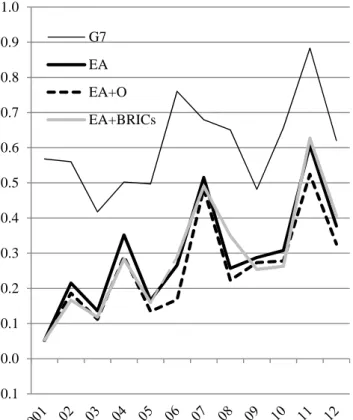
A number of economists have studied the impact of financial globalization on synchronization of economic variables such as business cycles and asset prices. Transmission of financial crisis or so-called crisis contagion is also directly related to the cross-border capital flows. Over the period of 2001-2012, a rise in stock market comovements is witnessed, particularly in the emerging Asian countries (EA henceforth); EA countries have near zero comovement in excess stock returns in early 2000s but the average correlation reached 0.4 in 2012 (Figure 1).1 Which factors can explain increased synchronization in stock market returns in EA? Is this the result of regional economic and financial integration among EA countries or increased capital flows between EA and advanced economies? Can this be an evidence of “coupling” or “decoupling” of Asian countries from the advanced economies?
This paper aims to account for the time-varying feature in the stock return synchronization among EA countries. In particular, we investigate the source of stock return comovements; bilateral capital flows among EA economies or synchronized capital flows from the advanced economies into EA economies. Stock market comovements shown in EA countries may indicate that there are increasing cross-border capital market transactions among EA countries. However, even without bilateral capital transactions, stock prices in EA countries can move together if capital flows from advanced economies to EA countries simultaneously. Identifying the source of stock market synchronization among EA countries is important to understand the nature of synchronization in financial markets in EA and to evaluate the impact of regional economic cooperation such as the Chiang Mai initiatives and Asian bond markets (Bekaert and Harvey, 2014).
Unlike previous studies that mainly relied on the price data to extract the common factors, we use the direct measure of cross-border financial flows using IMF’s CPIS (Coordinated Portfolio Investment Survey) data and estimate the effects of bilateral capital flows vs. third country effects from G7 countries in stock price comovements in EA countries.2 Impact of capital flows shocks from large countries on each EA countries should be different because of different degree of integration with the world financial markets.3 We capture those time-varying and country-specific effects of capital flows on stock prices by running dynamic panel regression using quantity data of capital flows.4
We make two contributions in the literature. First, since we focus on the post-financial liberalization period (2001-2012) in which EA financial markets are likely to be highly integrated with the rest of the world, we can capture the impact of non-institutional changes in economic
1 The average correlation among G7 countries is still higher around 0.6 in the same year.
2 Most previous papers use static or dynamic factor models to identify the shares of the variation in prices: national or global common factors (Bekaert et al., 2009; Forbes and Chinn, 2004).
3 Bekaert and Harvey (1997) argue that the correlations among national stock markets are directly linked to their degree of integration in the world capital market.
4 Some studies use quantity data of capital flows including Flavin et al. (2002), Froot and Ramadorai (2008) and Dellas and Hess (2005). However, they use cross-section or pooling regressions that neglects the time-dimension of the economic integration in the 2000s and beyond. Beine and Candelon (2011) and Bekaert and Wang (2009) use both time and cross-sectional dimensions simultaneously but they have limited focus on the effects of the degree of economic liberalization and openness.
3
globalization on excess stock market synchronization. Most previous research focused on the impact of liberalization in international financial markets on stock markets during the periods when financial markets are not completely liberalized.5 Based on the definition of “significant capital market liberalization timing” used in Bekaert (1995), all the countries in our sample have already finished their major capital account liberalization for the estimation period (Table 1). Thus, our analysis can capture the impact of cross-border capital flows arising from non-institutional economic reasons. Second, in empirical regressions, we control for potential problems of cross- sectional dependence, heteroscedasticity, and the possibility of serial correlation. We also control the endogeneity problems that arise from the dynamic nature of stock market comovements across countries (see, for instance, King et al., 1994 and Bekaert et al., 2009).
Baseline empirical analysis is conducted on pairs of 10 EA countries (thus 45 pairwise correlations a year) observed annually over the 2001–2012 period. We find that bilateral portfolio investment flows seem to explain stock price comovements in EA countries when included without the third country effects. However, the bilateral flow effects become insignificant when we include the third-country effects (portfolio investment from G7 countries to EA countries). The third country effects are highly significant and positive in most cases. Capital flows from G7 countries dominate the stock price movements in EA countries, even after controlling for potentially important factors such as trade agreements, industry difference, inflation, economic development, and financial depth.
Main conclusion of the regression results stands even when we extend the sample to including BRICs countries and FDI data. Therefore, we can claim that the “coupling” is still a reality in terms of stock returns in emerging markets.
The remainder of the paper is organized as follows. Section 2 describes the related literature and recent development in economic globalization of EA countries. Section 3 shows estimation models and variables used in the paper. Section 4 presents the main results of the empirical analysis with various sensitivity analyses. Section 5 concludes the paper.
2. Literature Review and the Economic Globalization in Emerging Asia
A large body of theoretical and empirical studies has focused on the role of real and financial linkages in explaining economic comovements. In regards to stock return comovements, previous studies in the 1990s find that the degree of comovements in emerging markets with the rest of the world is generally low, implying a limited impact of developed countries with large stock markets on small countries with emerging and developing markets (Bekaert and Harvey, 1997; De Santis &
Imrohoroglu, 1997; Forbes and Chinn, 2004). Behind the limited role are the presence of transaction costs such as restrictions on cross-country capital flows (e.g., Bekaert & Harvey, 2000) and the
5 See, for example, Bekaert and Harvey (1997, 2000), Bekaert et al. (2002), Dellas and Hess (2005), and Beine and Candelon (2011).
4
home bias in international investment (e.g., Karolyi and Stulz, 2003).
To measure the linkages of emerging markets with advanced economies, i.e. the third-country effects (for small countries), one strand of literature uses the international version of asset pricing models. Globally integrated financial markets make domestic stock returns partly determined by the covariance with the global returns.6 That is, global common shocks explain some portion of the variation of domestic stock returns. Several researchers empirically identify the global shocks by using factor models (e.g., Forbes and Chinn, 2004; Brooks and Del Negro, 2006), asset pricing models such as CAPM, the Fama-French model, APT models, and the Heston-Rouwenhorst model (e.g., Bekaert et al., 2009; Dutt and Mihov, 2013; Brooks and Del Negro, 2004, 2005).7 Advantage of this methodology is that one can identify the global factor(s), country-specific factor(s), and some other factor(s) such as sector-specific and regional factors from each country’s market returns without relevant measures of cross-border quantitative linkages among the sample countries.
Under the global markets, however, one should be cautious about the possibly increasing role of bilateral flows (bilateral effects) among emerging markets to correctly measure the third-country effects. Previous studies have not focused on the role of bilateral effects probably because of the lack of financial data and the limited size of bilateral flows in EA. It is difficult to isolate the bilateral effects of bilateral transactions from overall capital flows even with various measures of bilateral transactions, since bilateral linkages are highly correlated with other flow measures and also the spurious regression should be corrected (Forbes and Chinn, 2004).
Theoretical predictions about the influences of financial integration on comovements are a priori indeterminate. By generating large demand-side effects, financial linkages could create more synchronization at a first glance. However, financial linkages could also lead to more production specialization through reallocation of capital in different sectors. According to the international business cycle literature (Kalemli-Ozcan et al., 2013), financial globalization can result in more exposure to non-global shocks such as country-specific and sector-specific shocks, which can lower comovements.8 Forbes and Chinn (2004) present a nice example of indeterminacy. Consider a case that negative shocks in a large country g create a pessimistic view which drives down country g’s stock returns. One possible scenario is that this pessimistic view makes investors in country g contract their investment in a small country x to ensure their liquidity position, which lowers stock returns in country x (higher comovement). The other scenario is that investors in country g might shift exposure to a relatively better positioned country y and result in liquidity improvement only in country y, which can spur country y’s stock returns (lower comovements).
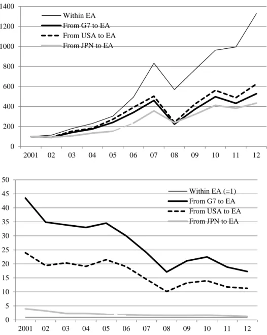
Figure 2 illustrates bilateral financial flows within EA countries and financial inflows from G7
6 The other strand is to use GARCH models and their variants which measure the share of stock price variation explained by global common factors as the degree of integration with the global markets. See, for example, Gérard et al. (2003).
7 For example, Forbes and Chinn (2004) run the regression of the computed country-specific factor loadings on several bilateral linkages between each small country and each large country. Bekaert et al. (2009) use asset pricing models and run various estimations with (excess) returns on stocks of each country on the left hand side and returns on global or developed countries’
portfolios on the right hand side.
8 Davis (2014) shows transmission through integrated equity markets create wealth effects that lead to lower comovements.
5
countries into EA countries. Bilateral financial flows within EA countries has risen by more than 13 times in terms of nominal values and that of financial inflows from G7 has risen by more than 5 times from 2001 to 2012. However, the absolute amount of financial inflows from G7 is still far much larger than that of bilateral financial flows within EA countries. These facts imply that the quantitative influence of G7 (particularly from the US) on the EA countries is still strong. However, the degree of influence can be changing over time and therefore, leaving aside the time dimension may lead to an incorrect interpretation.
Table 2 lists the total stock market capitalization of the sample 10 EA and G7 countries. From 2001 to 2012, the share of 10 EA countries in the world stock market has increased by more than 10% points, while the share of G7 countries has decreased by 25% points. The aggregated shares of 10 EA + G7 countries in the world are 88% in 2001 and 75% in 2012. On the other hand, the share of G7 countries alone has shrined from 81% in 2001 to 57% in 2012. Summing up the properties of the stock market and financial flows data, the presence of stock markets in 10 EA countries has emerged and those in G7 countries has declined, but capital inflows from G7 countries into EA are still large.
3. Empirical Estimation 3.1. Estimation Models
We first estimate the following static regression model:
, , , (1)
where , is pairwise excess stock return correlation , , is a set of bilateral financial flows between countries j and k and third-country effects from large country g to small countries j and k, , is a set of control variables. The error terms are = , where , , and represent a country-pairwise fixed effect that captures country-pair specific factor explaining comovements, year dummies, and the pure error terms, respectively.
This static model, however, does not capture potential dynamics of stock return comovements.
Therefore, we also use the following dynamic model with lagged dependent variable on the right hand side:
, , , , (2)
As described in Blundell and Bond (1998), Rioja and Valev (2004), and Wintoki (2012), this model itself involves some problems such as consistency and bias problems and possible simultaneity of explanatory variables. To solve those problems, we use system GMM (Blundell and Bond, 1998; Arellano and Bover, 1995):
, ,
, ,
, ,
,
, 0 (3)
with the assumption of following orthogonality conditions:
6
, , , 0,
, , , 0, for
s>1
(4)
The system GMM estimator can control for unobservable heterogeneity bias, inconsistency, and simultaneity, which enables us to produce efficient estimates. We use the lagged variables as instruments for estimating the system. Predetermined and endogenous variables in levels are instrumented with lagged levels and lagged first differences of their own. The model is estimated by two-step GMM whose estimates are asymptotically more efficient than those by one-step GMM.
3.2. Measures of Excess Stock Return Correlation
Variables used in the estimation and the data sources are all described in Table 3. Excess stock returns are computed from the U.S. dollar denominated stock returns over 3-month risk-free US T- bill rate. Following Bekaert et al. (2009), we use the weekly stock returns computed from national stock indices in order to avoid potential econometric problems of errors by non-synchronous trading of securities, which arises when using very highly frequent data. The indices are chosen from the list at the Bloomberg’s Indexes by Location. If multiple indices are listed for one country, one of them is chosen based on the data availability. We use the annual frequency pairwise correlation coefficients calculated from the computed weekly excess returns over about 52 weeks. Pairwise correlation coefficients ( ) between countries j and k are all Fisher’s z-transformed to avoid the limited dependent variable problem.9
3.3. Measures of Cross-Border Financial Flows
Measuring the degree of bilateral financial integration has been a challenge to many economists.
Previous studies have used the degree of restrictions on cross-border financial transactions (Kose et al., 2009) and non-bilateral measures of financial openness (Dellas and Hess, 2005). However, these measures capture the restrictions only on de jure financial flows (Imbs, 2006) and can cause identification problem for the sources of financial transactions. Moreover, as mentioned earlier, de jure restrictions in capital flows are relatively limited during our sample period. Therefore, we use the quantity-based financial integration data based on CPIS compiled by the IMF, which measures direct bilateral asset holdings. The data is available from 2001 which restricts our sample period from 2001-2012.10 CPIS data have covered portfolio investment only but recently started to release
9 Simple correlation coefficients can be non-constant over time as they are subject to the amplified effect during the period of high market volatility (Forbes and Rigobon, 2002). One way to tackle this problem is to use conditional correlation. Bekaert et al. (2009) claim that factor models can capture the expected correlation and the leftover error terms (if >0) can be considered as the effect of contagion that hikes volatility (and simple correlation coefficients). Another method is to control for the impact of time-variant interdependence among equity markets, which is the most important time-variant transmission channel of stock prices that can cause volatility (Longin and Solnik, 1995). The concept of this paper’s approach is similar to the latter approach.
10 CPIS reports bilateral equity holdings and debt securities holdings separately but due to numerous missing data, we focus on aggregate portfolio investment only. As Imbs (2006) documented, the components of CPIS (equity and debt investments) are strongly correlated with each other and the share of equity transaction is much larger than debt transaction in our sample.
7
FDI data since 2009. Later, we use the capital flows data including FDI for checking the sensitivity of the baseline results.
Bilateral financial flows between countries j and k (defined as bilateral effects) are measured as , where denotes holdings of country k’s portfolio investment by country j’s residents, vice versa. Y denotes GDP of each country. We also use the measure that includes FDI which is defined as , where denotes holdings of country k’s direct investment by country j’s residents, and vice versa. Due to the data availability of direct investment, we use the average of during period t’ (from 2009 to 2012) for the FDI measure for all periods.
Capital flows from G7 countries (named as g) to a pair of EA countries j and k (defined as third‐
country effects) are measured as , where ( denotes holdings of country j’s (k’s) portfolio investment by a third country g’s residents, and vice versa. We include only portfolio investment liabilities for each country (amount invested by G7 country g into country j, ), not portfolio investment asset (amount invested in G7 country g by country j, ) as the data show that many data points in portfolio investment assets are missing and even if they exist, the absolute amount is small.11 The third country measures that include FDI can be constructed by adding FDI from G7 country g into each pair of sample countries.
3.4. Control Variables
Several variables that are not seemingly related to capital flows can affect stock market comovements. In order to control for the omitted variable bias, a vector of control variables are included.
First, the literature often stresses the importance of economic fundamentals, particularly the role of industry structure. Roll (1992) claims that similar industrial compositions can generate a higher correlation in stock returns. However, Heston and Rouwenhorst (1994) found no significant role of industrial structure on stock return comovements by using an in-depth analysis of the data. More recently, Dutt and Mihov (2013) use time-varying country-pair–specific industrial composition measures and confirm the findings of Roll (1992). In this paper, following Imbs (2006), we use the so-called Krugman index (Krugman, 1991) to measure the similarity in industry specialization (defined as sectoral difference), ∑ where and denote the output shares of ISIC 1 digit-level industry n of countries j and k, respectively. The data is taken from United Nations’s Statistical Yearbook that covers all seven sectors. The expected sign of the estimated coefficient for this variable is negative. If countries j and k have similar industrial
11 In empirical estimation, we also use the data that include portfolio investment assets but the results are similar to the case when we use portfolio liabilities only.
8
structure, then the sectoral difference index would be smaller, while sector-specific shocks would move stock returns of both countries in the same direction and therefore create a high correlation of stock returns.
Second, the role of multilateral trade liberalization is considered. Theoretically, by lowering the cost of imported inputs, trade liberalization can increase expected future stock returns of countries that join the regional trade agreements, thereby increasing synchronization of stock returns (Basu and Morey, 1998). Previous research found that this theoretical prediction is empirically supported (Henry, 2000; Berben and Jansen, 2005). We use a dummy variable that takes 1 when a pair of countries has bilateral regional trade agreements (RTA). The expected sign on the coefficient is positive.
Third, we use three other variables to control for different macroeconomic fundamentals of countries in each pair: (1) pairwise sum of logged real per-capita GDP in US dollar (Economic Development) as the proxy for economic development of each pair of countries, (2) absolute difference in annual changes in CPI (Inflation Difference) as the proxy for differences in inflation rates of each pair of countries, and (3) the sum of ratios of domestic credit to private sector to output (Financial Development) as the proxy for the degree of availability of domestic financial intermediation. The expected signs of economic development, inflation difference, and financial development are positive, negative, and positive, respectively.
4. Estimation Results 4.1. Test for Strict Exogeneity
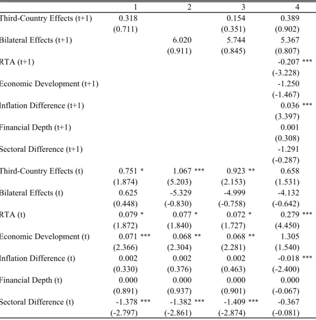
Before estimating the model, we test the strict exogeneity of capital flows data by examining whether bilateral effects and the third-country effects are related to the past stock price comovements. Theoretically, stock return comovements might lead to increased or decreased third country effects. From the perspective of portfolio diversification, if two countries exhibit similar stock price movements, there is less incentive for investors to increase investment in both countries at the same time, implying negative effects of stock price comovements on the third country effects.
However, information cascade in crisis contagion theory suggests that advanced economies might classify two small countries that show similar stock price movements in the same investment category and simultaneously change investment flows into these countries, which means positive effects of stock price comovements on the third country effects.
Following Wooldridge (2002), we run the following panel regression to test strict exogeneity.
(6) where is a subset of the bilateral and third-country effects and control variables at t+1, is the bilateral and third-country effects and control variables at t, and Yt is the pairwise correlation of stock prices. The null hypothesis of strict exogeneity is that is near zero and insignificant, since
9
stock price comovements should not be correlated with future realization of a subset of the bilateral and third-country effects and control variables.
Table 4 shows that the coefficient estimates for the future values of the bilateral and third- country effects are all statistically insignificant, indicating that they are strictly exogenous. This is also the case with control variables. Note that the future values of RTA and inflation difference are significantly different from zero, but their signs are opposite to the theoretically predicted value.
Given these results, all explanatory variables are assumed to be strictly exogenous (and lagged is endogenous). In the sensitivity analysis, we examine the case assuming the bilateral effects are predetermined.
4.2. Baseline Estimation
Table 5 reports the regression results of the baseline model. We first examine the model with bilateral effects only (first four columns) and then the models with both bilateral and third country effects (last four columns). We use both static and dynamic panel regression models for two sets of control variables (with and without financial depth and sectoral difference variables, while RTA, economic development and inflation difference are always included). For static regression model, the standard Hausman tests support the use of random effects models. For dynamic regression model, one year lag of dependent variable is included in the regression, while two and three years of lags are used as instruments.12
We find several important observations from the regressions. The coefficients on bilateral portfolio investment flows are marginally significant when excluding the third country effects. The coefficients are positive implying that higher bilateral financial flows increase stock return comovements in the EA countries. However, the positive effects of bilateral financial flows disappear when the third country effects are included. In the regressions with both bilateral and third country effects, the bilateral financial flows become all insignificant with negative signs in some cases, while the third country effects are all positive and significant with the 1% level. These results are consistent in both static and dynamic models and also in both control variable sets.
This result strongly supports that the positive stock return comovements in EA countries are mainly due to capital flows from G7 countries, not from bilateral financial flows among EA countries. This finding is similar to those obtained by prior studies using different methodologies (Forbes and Chinn, 2004; Dellas and Hess, 2005; Froot and Ramadorai, 2008). When all five control variables are used, the positive effects of G7 capital flows become stronger compared to the case
12 We provide various test statistics of the dynamic models in the bottom panel of Table 5. The specification tests with AR(1) and AR(2) serial correlations show p-values of 0.00 and 0.23 ~ 0.32, respectively, which indicates that the null hypothesis of no 2nd order serial correlation cannot be rejected. For the Hansen J statistic of over-identification restrictions, the robust minimized value of the two-step GMM criterion function displays the p-value of 0.67, implying that the hypothesis that our instruments are valid cannot be rejected. As discussed earlier, the system GMM estimator (dynamic models) makes an additional exogeneity assumption: the assumption that any correlation between our endogenous variables and the unobserved (fixed) effect is constant over time. This is the assumption that enables us to include the levels equations in the dynamic models and use lagged differences as instruments for these levels. For the test on the exogeneity of the instruments, we use the difference-in-Hansen test of exogeneity (See Eichenbaum et al., 1988). The p-value for the J-statistic is 0.10 ~ 0.59 and the null hypothesis of exogeneity cannot be rejected.
10
with only three control variables. There can be some explanations behind the insignificant coefficients on bilateral capital flows. Regional integration of financial markets in EA countries is still under progress and the actual amount of financial flows among EA countries are quite small compared to capital flows from G7 countries to EA countries (Figure 2). That is, EA financial markets are more integrated with the US and other G7 markets than among regional countries.
Therefore, bilateral capital flows among EA countries do not explain stock price correlations, while the third-country effects in capital flows significantly affect stock price correlation.
Coefficients on control variables seem to make sense in most cases. Coefficient on economic development is positive and significant, implying that rich country pairs in the region tend to have high stock return correlation. About the sectoral difference variable, all the coefficients are negative which is consistent with theoretical predictions but are mostly insignificant.13 The RTA variable has significant and positive influence on stock return comovements, consistent with theoretical predictions that having a common free-trade agreement leads to higher stock return correlations (Dutt and Mihov, 2013).14 Financial depth and sectoral difference data are mostly insignificant.
4.3. Sensitivity Analysis
We are interested in which country among G7 countries has the significant effects on stock return comovements in EA region. Tables 6 displays the regression results when we replace G7 countries with USA, Japan, and the sum of four European countries (France, Germany, Italy, UK), respectively. In all case, the coefficients on the third country effects are significant and positive, implying that we cannot exclude any single country among G7 in estimating the third country effects. Bilateral effects are all insignificant and the signs of coefficients are positive in the static models and negative in the dynamic models. Coefficients on control variables are similar in all cases.
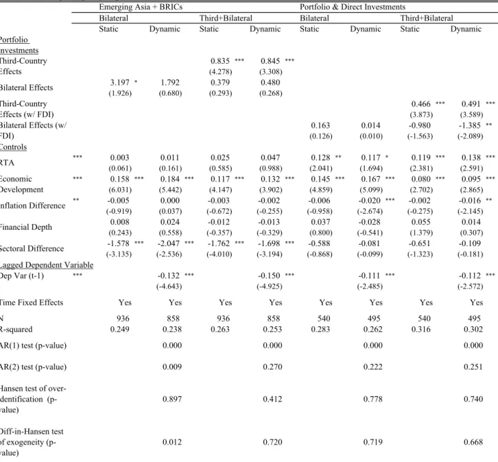
We extend the analysis to other emerging markets in other regions. The first four columns of Table 7 shows the case when we extend the sample countries to 10 EA countries plus non-Asian BRICs countries such as Brazil, Russia, and South Africa. Now, with 13 countries, we have 78 country pairs for 12 year sample periods, total 936 sample size which is an increase from 540 in the previous case with only EA countries. With BRICs in the sample, main conclusion still holds: third- country effects are positive and significant. Bilateral effects are insignificant in most cases. One interesting finding is that the sectoral difference now has significant and negative effects on comovements. Because the newly included countries have different industry structure from EA countries, sectoral differences are much more present in the sample data, which can explain a significant and negative coefficient.
13 This might be due to a rough sectoral classification that we used. Introducing more sophisticated measures such as in Dutt and Mihov (2013) may produce different results.
14 Some previous research used trade flows as explanatory variables, such as Forbes and Chinn (2004) and Walti (2011). However, the coefficients are sometimes not significant and negative. Theoretically, the effects of trade flows on stock return comovements can be either way, depending on the types of trade. In this paper, we do not explicitly include trade flows because of endogeneity issue, especially with RTA and industry structure. The endogeneity issue is well documented in Beine and Candelon (2011) and Lane and Milesi-Ferretti (2008).
11
The last four columns in Tables 7 reports the case when we expand the capital flows data including FDI. Inclusion of FDI in capital flows data is theoretically and empirically important (Imbs, 2006; Otto et al., 2001). Ideally, it would be better to consider portfolio investment and FDI separately. However, due to the lack of time-series data for FDI (available only from 2009), we can add FDI data to portfolio investment data only for a subset of years. The empirical results show that the main results still hold with FDI data included; the third country effects are significant and positive. The actual size of coefficients decrease but this is due to the fact that capital flows data are now larger including FDI.
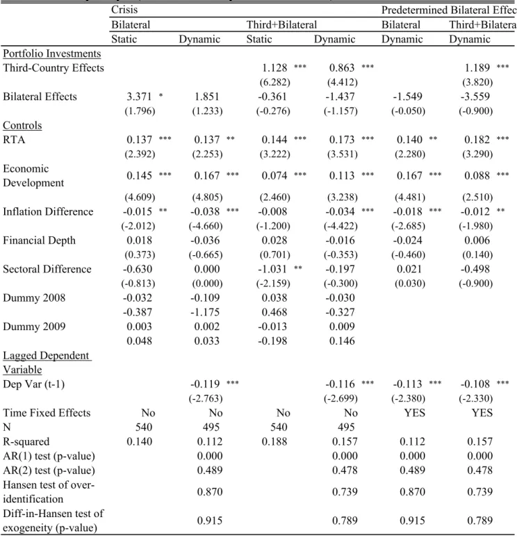
Finally, Table 8 displays two additional sensitivity studies; first case without time fixed effects but including financial crisis dummies (2008, 2009=1, otherwise 0) and the second case with assuming bilateral effects that are predetermined. Both cases show that the main conclusion stands.
5. Conclusion
The objective of this paper is to analyze the sources of stock return synchronization in EA countries, whether it is due to increased bilateral capital flows among EA countries or synchronized capital flows from G7 economies into EA countries. The regression results show that the main force behind stock return comovements in EA is the third country effects, not bilateral capital flows. There has been a serious progress in Asian financial market integration in recent years due to various types of regional economic and financial cooperation including the Chiang Main Initiative and development of the Asian Bond Markets. However, empirical analysis in this paper shows that the size of capital flows among EA countries is still small and does not have significant effects on stock market return movements. A majority of stock return comovements is still explained by capital flows from G7 countries.
The results from various models in this paper point to the necessity of a deeper study of sources of stock return comovements in the emerging Asian countries. First, in addition to portfolio investments and FDI, the role of global bank lending channels can be important to pin down the third-country effects more comprehensively (Kalemli-Ozcan et al., 2013). Second, measuring the third-country effects in a large set of countries requires careful assessment of control variables.
Without proper control variables, we may get biased results. Third, uncertainty shocks can play an important role in explaining asset price comovements (Hirata et al., 2013), although creating such uncertainty measures for emerging economies can be a challenge.
12 References
Andersen, T.G., T. Bollerslev, F.X. Diebold, and P. Labys. 2003, “Modeling and Forecasting Realized Volatility.”
Econometrica, 71, 579–625.
Basu, P., and M. R. Morey. 2005. “Trade Opening and the Behavior of Emerging Stock Market Prices.” Journal of Economic Integration, 20, 68-92.
Beine, M., and B. Candelon. 2011. “Liberalisation and Stock Market Co-Movement between Emerging Economies.”
Quantitative Finance, 11(2), 299-312.
Bekaert, G. 1995. “Market Integration and Investrnent Barriers in Emerging Equity Markets.” World Bank Economic Review, 9, 75-107.
Bekaert, G., and C. R. Harvey. 1997. “Emerging Equity Market Volatility.” Journal of Financial Economics, 43, 29- 77.
Bekaert, G., and C. R. Harvey. 2000. “Foreign Speculators and Emerging Equity Markets.” The Journal of Finance, 55(2): 565-613.
Bekaert, G., and C. R. Harvey. 2002. “Research in Emerging Markets Finance: Looking to the Future.” Emerging Markets Review, 3, 429-448.
Bekaert, G., and C. R. Harvey. 2014. “Emerging Equity Markets in a Globalizing World.” mimeo.
Bekaert, G., C. R. Harvey, and R. L. Lumsdaine. 2002. “The Dynamics of Emerging Market Equity Flows.” Journal of International Money and Finance, 21(3), 295-350.
Bekaert, G., C. R. Harvey, and R. L. Lumsdaine. 2005. “Does Financial Liberalization Spur Growth?” Journal of Financial Economics, 77, 3-55.
Bekaert, G., R. J. Hodrick, and X. Zhang. 2009. “International Stock Return Comovements.” The Journal of Finance, 64(6): 2591-2626.
Bekaert, G., and X. S. Wang. 2009. “Globalization and Asset Prices.” Mimeo.
Berben, R.P., and W.J. Jansen. 2005. “Comovement in International Equity Markets: A Sectoral View.” Journal of International Money and Finance, 24, 832-857.
Blundell, R. and S. Bond, 1998. “Initial Conditions and Moment Restrictions in Dynamic Panel Data Models.”
Journal of Econometrics, 87, 115–143.
Brooks, R., and M. Del Negro. 2004. “The Rise in Comovement Across National Stock Markets: Market Integration or IT Bubble?” Journal of Empirical Finance, 11(5): 659-680.
Brooks, R., and M. Del Negro. 2005. “Country Versus Region Effects in International Stock Returns.” The Journal of Portfolio Management, 31(4): 67-72.
Brooks, R., and M. Del Negro. 2006. “Firm-Level Evidence on International Stock Market Comovement.” Review of Finance, 10(1): 69-98.
Davis, J. S. 2014. “Financial Integration and International Business Cycle Co-movements.” Journal of Monetary Economics, 64, 99-111.
Dellas, H., and M. Hess. 2005. “Financial Development and Stock Returns: A Cross-Country Analysis.” Journal of International Money and Finance, 24(5): 891-912.
De Santis, G., and S. Imrohoroglu, 1997. “Stock returns and volatility in emerging financial markets.” Journal of International Money and Finance, 16(4), 561-579.
Dutt, P., and Mihov, I. “Stock Market Comovements and Industrial Structure.” Journal of Money, Credit and Banking, 45(5), 891-911.
Eichenbaum, M. S., L. P. Hansen, and K. J. Singleton. 1988. “A Time Series Analysis of Representative Agent Models of Consumption and Leisure Choice under Uncertainty.” Quarterly Journal of Economics, 103, 51–78.
Flavin, T. J., M. J. Hurley, and F. Rousseau. 2002. “Explaining Stock Market Correlation: A Gravity Model Approach” The Manchester School Supplement, 70: 87-106.
Forbes, K. J., and M. D. Chinn. 2004. “A Decomposition of Global Linkages in Financial Markets Over Time” The Review of Economics and Statistics, 86(3): 705-722.
Forbes, K. J., and R. Rigobon. 2002. “No Contagion, Only Interdependence: Measuring Stock Market Comovements” The Journal of Finance, 57(5): 2223-2261.
Froot, K. A., and T. Ramadorai. 2008 “Institutional Portfolio Flows, International Investments.” The Review of Financial Studies, 21(2), 937-971.
Gérard, B., K. Thanyalakpark, and J. A. Batten. 2003. “Are the East Asian Markets Integrated? Evidence from the ICAPM.” Journal of Economics and Business, 55, 585–607.
Henry, Peter B., 2000. “Stock Market Liberalization, Economic Reform, and Emerging Market Equity Prices.”
Journal of Finance, 55(2), 529-564.
Heston, S. L., and K. G. Rouwenhorst. 1994 “Does Industrial Structure Explain the Benefits of International Diversification?” Journal of Financial Economics, 46, 111–157.
Hirata, H., M. A. Kose, C. Otrok, and M. Terrones. 2013. “Global House Price Fluctuations: Synchronization and Determinants.” NBER International Seminar on Macroeconomics 2012, University of Chicago Press, 119-166.
13
Imbs, J. 2006. “The Real Effects of Financial Integration” Journal of International Economics, 68(2): 296-324.
Karolyi, G. D., and R. M. Stulz .1996. “Why Do Markets Move Together? An Investigation of US-Japan Stock Return Comovements.” Journal of Finance. 51(3), 951-986.
King, M., E. Sentana, and S. Wadhwani. 1994. “Volatility and Links between National Stock Markets.”
Econometrica, 62(4), 901-933.
Kose, M. A., E. S. Prasad, and M. E. Terrones. 2009. Does Openness to International Financial Flows Raise Productivity Growth? Journal of International Money and Finance, 28, 554–580.
Krugman, P. R. 1991. “Increasing Returns and Economic Geography.” Journal of Political Economy, 99 (3), 483- 499.
Lane, P. R., and G. M. Milesi-Ferretti, 2008, “The Drivers of Financial Globalization.” American Economic Review, 98 (2), 327-332.
Otto, G., G. Voss, and L. Willard. 2001. “Understanding OECD Output Correlations.” RBA Research Discussion Papers, 2001-05.
Rioja, F., and N. Valev. “Does One Size Fit All?: a Reexamination of the Finance and Growth Relationship.”
Journal of Development Economics, 74, 429–447.
Roll, R., 1992. “Industrial Structure and the Comparative Behavior of International Stock Market Indices.” Journal of Finance, 47, 3–41.
Kalemli-Ozcan, S., E. Papaioannou, and J-L. Peydro. 2013. “Financial Regulation, Financial Globalization, and the Synchronization of Economic Activity.” Journal of Finance (3) 1179-1228
Walti, S. “Stock Market Synchronization and Monetary Integration.” 2011. Journal of International Money and Finance, 30, 96–110
Wintoki, M. B., J. S. Linck, and J. M. Netter, “Endogeneity and the Dynamics of Internal Corporate Governance.”
Journal of Financial Economics, 105, 581-606.
Wooldridge, J.M., 2002. Econometric Analysis of Cross Section and Panel Data. The MIT Press, Cambridge.
14
Figure 1. Average Stock Return Correlation in G7 and EA Countries
Note: The figure draws equally weighted average annual pairwise correlation of excess stock returns in G7 countries, 10 EA countries, EA+ 2 Oceania countries (EA+O), and EA+ 3 non-EA BRICs countries (EA+BRICs). See Table 1 for detailed country information. The correlation coefficients are computed from weekly US dollar denominated excess returns on stocks over the U.S. T-bill rate.
-0.1 0.0 0.1 0.2 0.3 0.4 0.5 0.6 0.7 0.8 0.9 1.0
G7 EA EA+O EA+BRICs
15
Figure 2. Financial Flows within EA countries and Inflows from G7
Note: The figure draws bilateral financial flows (portfolio investment) within EA countries and financial inflows from G7 countries (USA, and Japan) into EA countries. The top chart draws the graphs as indices (1990=100) and the bottom chart draws the graphs by setting bilateral financial flows within EA countries as one in each year.
0 200 400 600 800 1000 1200 1400
2001 02 03 04 05 06 07 08 09 10 11 12
Within EA From G7 to EA From USA to EA From JPN to EA
0 5 10 15 20 25 30 35 40 45 50
2001 02 03 04 05 06 07 08 09 10 11 12
Within EA (=1) From G7 to EA From USA to EA From JPN to EA
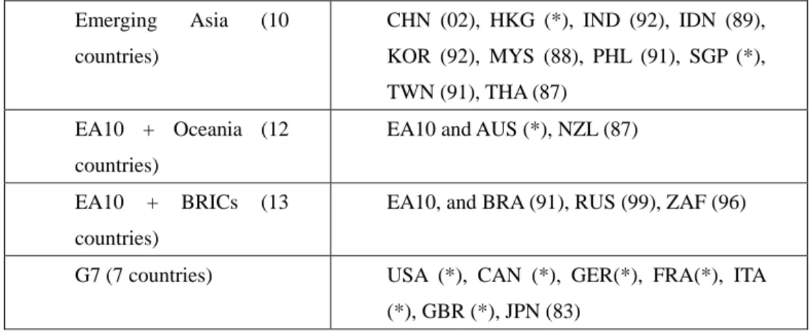
16 Table 1. Sample Countries
Emerging Asia (10 countries)
CHN (02), HKG (*), IND (92), IDN (89), KOR (92), MYS (88), PHL (91), SGP (*), TWN (91), THA (87)
EA10 + Oceania (12 countries)
EA10 and AUS (*), NZL (87)
EA10 + BRICs (13 countries)
EA10, and BRA (91), RUS (99), ZAF (96)
G7 (7 countries) USA (*), CAN (*), GER(*), FRA(*), ITA (*), GBR (*), JPN (83)
Note: Numbers in brackets are years when domestic stock market is liberalized for foreign investors (Bekaert and Harvey, 2000 and 2002, Bekaert, Harvey, and Lundblad, 2005). * indicates that the country considered is already fully liberalized when these studies are conducted.
Table 2. Stock Market Share in sample years
Note: Numbers are shares of each country’s total market capitalization in the world. Data sources are International Financial Data and Taiwan Stock Exchange. BRICs include not only non-EA BRICs (BRA, RUS, ZAF) but also EA BRICs (CHN, IND).
Oceania
Emerging
Asia BRICs G7
USA JPN
2001 1.5% 7.4% 3.9% 81.2% 51.7% 8.4%
2005 2.1% 9.7% 7.1% 73.3% 41.4% 11.6%
2008 2.2% 19.2% 15.2% 64.5% 36.2% 9.9%
2010 2.8% 19.9% 17.4% 55.0% 31.2% 7.5%
2012 2.5% 18.2% 14.1% 57.1% 34.2% 6.7%
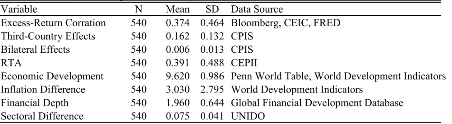
Table 3. Variables, Summary Statistics, and Data Sources
Variable N Mean SD Data Source
Excess-Return Corration 540 0.374 0.464 Bloomberg, CEIC, FRED Third-Country Effects 540 0.162 0.132 CPIS
Bilateral Effects 540 0.006 0.013 CPIS
RTA 540 0.391 0.488 CEPII
Economic Development 540 9.620 0.986 Penn World Table, World Development Indicators Inflation Difference 540 3.030 2.795 World Development Indicators
Financial Depth 540 1.960 0.644 Global Financial Development Database Sectoral Difference 540 0.075 0.041 UNIDO
Table 4. Testing Strict Exogeneity
1 2 3 4
Third-Country Effects (t+1) 0.318 0.154 0.389
(0.711) (0.351) (0.902)
Bilateral Effects (t+1) 6.020 5.744 5.367
(0.911) (0.845) (0.807)
RTA (t+1) -0.207***
(-3.228)
Economic Development (t+1) -1.250
(-1.467)
Inflation Difference (t+1) 0.036 ***
(3.397)
Financial Depth (t+1) 0.001
(0.308)
Sectoral Difference (t+1) -1.291
(-0.287) Third-Country Effects (t) 0.751 * 1.067 *** 0.923** 0.658
(1.874) (5.203) (2.153) (1.531)
Bilateral Effects (t) 0.625 -5.329 -4.999 -4.132
(0.448) (-0.830) (-0.758) (-0.642)
RTA (t) 0.079 * 0.077 * 0.072* 0.279 ***
(1.872) (1.840) (1.727) (4.450)
Economic Development (t) 0.071 *** 0.068 ** 0.068** 1.305
(2.366) (2.304) (2.281) (1.540)
Inflation Difference (t) 0.002 0.002 0.002 -0.018***
(0.330) (0.376) (0.463) (-2.400)
Financial Depth (t) 0.000 0.000 0.000 0.000
(0.891) (0.937) (0.901) (-0.067)
Sectoral Difference (t) -1.378*** -1.382*** -1.409*** -0.367 (-2.797) (-2.861) (-2.874) (-0.081)
Table 5. Stock Market Correlations Regressions
Portfolio Investments
1.066 *** 1.000 *** 1.119 *** 1.087 ***
(6.428) (5.251) (5.974) (5.255)
3.653 ** 3.330 * 3.146 2.921 * 0.277 -0.101 -0.987 -1.154
(2.099) (1.849) (1.610) (1.750) (0.228) (-0.087) (-0.760) (-0.985)
Controls
0.101 * 0.109 ** 0.093 0.114 ** 0.120 *** 0.139 *** 0.157 *** 0.167 ***
(1.851) (2.289) (1.479) (2.269) (2.983) (3.375) (3.518) (3.783)
0.127 *** 0.128 *** 0.156 *** 0.137 *** 0.068 *** 0.069 *** 0.085 *** 0.078 ***
(4.224) (5.569) (4.617) (4.886) (2.366) (2.829) (2.645) (2.713)
-0.004 -0.007 -0.008 -0.018 *** 0.001 -0.005 -0.014 * -0.015 **
(-0.676) (-1.243) (-0.394) (-2.476) (0.112) (-0.836) (-1.942) (-2.255)
0.032 -0.028 0.033 0.002
(0.713) (-0.452) (0.904) (0.057)
-0.705 -0.450 -1.113 *** -0.609
(-1.045) (-0.518) (-2.567) (-1.119)
Lagged Dependent Variable
Dep Var (t-1) -0.139 *** -0.118 *** -0.113 *** -0.113 ***
(-2.480) (-2.794) (-2.560) (-2.607)
Constant Yes Yes Yes Yes Yes Yes Yes Yes
Time Fixed
Effects Yes Yes Yes Yes Yes Yes Yes Yes
N 540 540 495 495 540 540 495 495
R-squared 0.293 0.291 0.273 0.275 0.337 0.331 0.271 0.314
AR(1) test (p-
value) 0.000 0.000 0.000 0.000
AR(2) test (p-
value) 0.318 0.288 0.232 0.291
Hansen test of over-
identification (p- value)
0.292 0.668 0.707 0.667
Diff-in-Hansen test of exogeneity (p- value)
0.109 0.591 0.604 0.591
Bilateral Effects + Third-country Effects Bilateral Effects
Economic Development RTA
Inflation Difference Financial Depth Sectoral Difference
Dynamic Models
Bilateral Effects Third-Country Effects
Static Models Dynamic Models Static Models
Table 6. Third Country Effects by Country/Region
Portfolio Investments
1.799 *** 1.755 ***
(6.514) (5.629)
9.120 *** 13.573 ***
(3.750) (4.618)
3.021 *** 4.353 ***
(5.966) (5.261)
0.385 -0.684 0.059 -2.559 1.242 -1.072
(0.327) (-0.566) (0.045) (-1.415) (0.958) (-0.748)
Controls
0.125 *** 0.163 *** 0.099 ** 0.121 *** 0.106 *** 0.149 ***
(3.108) (3.547) (2.276) (2.747) (2.573) (3.648)
0.064 ** 0.085 *** 0.090 *** 0.088 ** 0.084 *** 0.087 ***
(2.171) (2.579) (2.736) (2.297) (3.222) (2.753)
0.001 -0.013 * 0.001 -0.011 -0.002 -0.015 **
(0.232) (-1.926) (0.084) (-1.609) (-0.270) (-2.126)
0.033 0.004 0.049 0.021 0.026 -0.007
(0.909) (0.095) (1.172) (0.426) (0.724) (-0.159)
-0.975 *** -0.455 -1.222 *** -0.968 * -1.187 *** -0.842
(-2.332) (-0.837) (-2.523) (-1.648) (-2.596) (-1.539)
Lagged Dependent Variable
-0.112 *** -0.113 *** -0.114 ***
(-2.546) (-2.465) (-2.622)
Constant Yes Yes Yes Yes Yes Yes
Time Fixed Effects Yes Yes Yes Yes Yes Yes
N 540 495 540 495 540 495
R-squared 0.335 0.319 0.316 0.302 0.327 0.321
AR(1) test (p-value) 0.000 0.000 0.000
AR(2) test (p-value) 0.288 0.345 0.265
Hansen test of over- identification (p- value)
0.629 0.670 0.771
Diff-in-Hansen test of
exogeneity (p-value) 0.565 0.632 0.665
Third-country Effects from
Third-country Effects (USA)
Third-country Effects (Japan)
Third-country Effects (Europe)
Bilateral Effects
RTA Economic Development Inflation Difference Financial Depth Sectoral Difference
Dep Var (t-1)
Dynamic Europe Japan
USA
Static Dynamic Static Dynamic Static
Table 7. Sensitivity Analysis (Sample Countries, Definition of Investments)
Bilateral Third+Bilateral Bilateral Third+Bilateral
Static Dynamic Static Dynamic Static Dynamic Static Dynamic
Portfolio Investments
0.835 *** 0.845 ***
(4.278) (3.308)
3.197 * 1.792 0.379 0.480
(1.926) (0.680) (0.293) (0.268)
0.466 *** 0.491 ***
(3.873) (3.589)
0.163 0.014 -0.980 -1.385 **
(0.126) (0.010) (-1.563) (-2.089)
Controls
*** 0.003 0.011 0.025 0.047 0.128 ** 0.117 * 0.119 *** 0.138 ***
(0.061) (0.161) (0.585) (0.988) (2.041) (1.694) (2.381) (2.591)
*** 0.158 *** 0.184 *** 0.117 *** 0.132 *** 0.145 *** 0.167 *** 0.080 *** 0.095 ***
(6.031) (5.442) (4.147) (3.902) (4.859) (5.099) (2.702) (2.865)
** -0.005 0.000 -0.003 -0.002 -0.006 -0.020 *** -0.002 -0.016 **
(-0.919) (0.037) (-0.672) (-0.255) (-0.958) (-2.674) (-0.275) (-2.145)
0.008 0.024 -0.012 -0.013 0.037 -0.028 0.055 0.014
(0.243) (0.558) (-0.357) (-0.329) (0.800) (-0.541) (1.379) (0.307)
-1.578 *** -2.047 *** -1.762 *** -1.698 *** -0.588 -0.081 -0.651 -0.109
(-3.135) (-2.536) (-4.010) (-3.194) (-0.868) (-0.099) (-1.323) (-0.181)
Lagged Dependent Variable
Dep Var (t-1) *** -0.132 *** -0.150 *** -0.111 *** -0.112 ***
(-4.643) (-4.925) (-2.485) (-2.572)
Time Fixed Effects Yes Yes Yes Yes Yes Yes Yes Yes
N 936 858 936 858 540 495 540 495
R-squared 0.249 0.238 0.263 0.253 0.283 0.262 0.316 0.302
AR(1) test (p-value) 0.000 0.000 0.000 0.000
AR(2) test (p-value) 0.009 0.270 0.222 0.251
Hansen test of over- identification (p- value)
0.897 0.412 0.778 0.740
Diff-in-Hansen test of exogeneity (p- value)
0.012 0.720 0.719 0.668
Portfolio & Direct Investments Emerging Asia + BRICs
Third-Country Effects Bilateral Effects Third-Country Effects (w/ FDI) Bilateral Effects (w/
FDI)
RTA Economic Development Inflation Difference Financial Depth Sectoral Difference
Table 8. Sensitivity Analysis (Time Dummies only for the Crisis Period)
Predetermined Bilateral Effects
Bilateral Third+Bilateral Bilateral Third+Bilateral
Static Dynamic Static Dynamic Dynamic Dynamic
Portfolio Investments
Third-Country Effects 1.128 *** 0.863 *** 1.189 ***
(6.282) (4.412) (3.820)
Bilateral Effects 3.371 * 1.851 -0.361 -1.437 -1.549 -3.559
(1.796) (1.233) (-0.276) (-1.157) (-0.050) (-0.900)
Controls
RTA 0.137 *** 0.137 ** 0.144 *** 0.173 *** 0.140 ** 0.182 ***
(2.392) (2.253) (3.222) (3.531) (2.280) (3.290)
Economic
Development 0.145 *** 0.167 *** 0.074 *** 0.113 *** 0.167 *** 0.088 ***
(4.609) (4.805) (2.460) (3.238) (4.481) (2.510)
Inflation Difference -0.015 ** -0.038 *** -0.008 -0.034 *** -0.018 *** -0.012 **
(-2.012) (-4.660) (-1.200) (-4.422) (-2.685) (-1.980)
Financial Depth 0.018 -0.036 0.028 -0.016 -0.024 0.006
(0.373) (-0.665) (0.701) (-0.353) (-0.460) (0.140)
Sectoral Difference -0.630 0.000 -1.031 ** -0.197 0.021 -0.498
(-0.813) (0.000) (-2.159) (-0.300) (0.030) (-0.900)
Dummy 2008 -0.032 -0.109 0.038 -0.030
-0.387 -1.175 0.468 -0.327
Dummy 2009 0.003 0.002 -0.013 0.009
0.048 0.033 -0.198 0.146
Lagged Dependent Variable
Dep Var (t-1) -0.119 *** -0.116 *** -0.113 *** -0.108 ***
(-2.763) (-2.699) (-2.380) (-2.330)
Time Fixed Effects No No No No YES YES
N 540 495 540 495
R-squared 0.140 0.112 0.188 0.157 0.112 0.157
AR(1) test (p-value) 0.000 0.000 0.000 0.000
AR(2) test (p-value) 0.489 0.478 0.489 0.478
Hansen test of over-
identification 0.870 0.739 0.870 0.739
Diff-in-Hansen test of
exogeneity (p-value) 0.915 0.789 0.915 0.789
Crisis