水面に拘束されたバブルの運動の数値シミュレーション(非線形現象のモデル化とその数理解析)

水面に拘束されたバブルの運動の数値シミュレーション

Numerical

simulation of

motion

of

a

bubble

restrained

to water

surface

金沢大学 自然科学研究科山崎崇史 (YAMAZAKI, TAKASHI)

Graduate School of Natural Science and Technology,

Kanazawa University

金沢大学 自然科学研究科小俣正朗 (OMATA, SEIRO)

Graduate School of Natural Science and Technology,

Kanazawa University

金沢大学 自然科学研究科長山雅晴 (NAGAYAMA, MASAHARU)

Graduate School of Natural Science and Technology,

Kanazawa University

Abstract. The aim of this paper is to develop the numerical method for solving

the hyperbolic free-boundary problem under the volume conservation $\mathrm{c}\mathrm{o}\mathrm{n}\mathrm{s}\mathrm{t}\mathrm{r}\mathrm{a}\dot{\mathrm{i}}\mathrm{t}$

.

The

equation treated in this paper has

a

degenerate hyperbolic operator and non-local

term (Lagrange multiplier) coming from volume constraint. The typical phenomena

described by this equation

are

the motion of bubble

on water

surface and oil droplet

motion

on a

plane. Wetryto realize them numcricaly. It is the

method

called discrete

Morse

_flow

$(DMF)$

of

hyperbolic type that plays

an

important role in the numerical

simulation or the stage of construction ofan approximateweak solution. The DMF is

based

on

the variational method using time-semidiscretized functional and is suitable

to treat

a

volume constraint condition.

1

Introduction

In this paper,

we

treat numericallythe motionof a bubble which

moves

on a

water surface

or an

oil droplet

on a

flat plane. There

are some common

features in these phenomena. The

first common

feature

is that the volume does

not

changealong their

motion. The second

common

feature of these phenomena is that the

area

where the

bubble

or

oil droplet exist is localized. We call the set of points where the bubble touches the water surface

or

where the surface of oil droplet touches the plane $fi\epsilon e-$

boundary. In this section

we

explain the model equation that rules the motion ofthe

bubble. However, the model ofthe bubble

can

be applied also to the motionof the oil

droplet because ofthese two

common

properties.

We use the graph of

a

scalar function $u$ to describe the shape ofthe bubble. The

zero

level set of$u$coincideswith thewatersurface. Theset ofpoints wherethe bubble

touchcs the water surface is called free-boundary. In order to simplify the model,

we

assume

that the water layer is

so

thin that its flow

or

movement does not influence

tensor

density of

the

bubble and water

surface

to be homogeneous and isotropic.

We

also

assume

that the volume of air which is

surrounded

by the bubble is pre-served at

any

time, i.e., $\int_{\Omega}udx=M=\mathrm{c}\mathrm{o}\mathrm{n}\mathrm{s}\mathrm{t}.$

,

that is, the bubble movement

can

be

described by

wave

equation with volume constraint. The following equation describes

the phenomenawcll:

$\chi_{u>0}u_{tt}=\Delta u-R^{2}\chi_{\epsilon}’(u)+\lambda\chi_{u>0}$ _{$(x\in\Omega, 0<t<\tau)$}

.

(1.1)

Here $\Omega$ is

a

bounded domain in $\mathrm{R}^{m}$ (in the following, to simplify the notation, _{$\Omega_{\tau}=$}

$\Omega\cross(0,\tau)\subset \mathrm{R}^{m+1}$ is used), and _{$\chi_{u>0}$} is the characteristic

function of

the

set

_$\{u>0\}$

and

$\chi_{\epsilon}\in C^{2}(\mathrm{R})$ is

a

smoothing of$\chi$ satisfying

$\chi_{\epsilon}(s)=\{$

$0$, _{$s\leq 0$}

1, $\epsilon\leq s$

with interpolating in $0<s<\epsilon$ in such

a

way that

I

$\chi_{\epsilon}’(s)|\leq C/\epsilon$

.

The

term

$R^{2}\chi_{\epsilon}’(u)$

describes the net adhesive force.

It

is due to this rcstriction force that the generation of the

new

surface

or movement

offree-boundary

are

obstructed. The specificity of

equation (1.1) lies in the coefficient $\chi_{u>0}$

on

the left-hand side.

Bccause

of this

co-efficient, non-negativity of the solution is guaranteed.

Function

$\lambda$, which appears in

the last term of (1.1) is

a

Lagrange multiplier originating in the volume preservation

condition. The explicit formof the Lagrange multiplier A is obtained

as

follows:

$\lambda=\frac{1}{M}\int_{\Omega}[uu_{\ell t}\chi_{u>0}+|\nabla u|^{2}+R^{2}u\chi_{e}’(u)]dx$ (1.2)

by formal calculation with

volume

constraint under the assumption that

A

does not

depend

on space

variables. The integral representation of Lagrange multiplier makes

theproblem

more

difficult.

However,

we

can

calculate

an

approximatesolution to (1.1)

by

use

of

a

time-semidiscretized functional which is called the discre$te$

Morse

flow

of

hyperbolic type (see [7]).

2

Minimizing

method

for the bubble

problem

Like in [8], we introduce another approximation problem to (1.1). Here, we give

thevolume constraint in the admissible space for finding

a

minimizer of

a

discretized functional correspondingto the Lagrangian.

Problem

2.1.

Let $\Omega$ be a bounded domain in $\mathrm{R}^{m}$

.

For $n=2,3,$

$\ldots$

,

find

minimizer $u_{n}$

of

the follouring

functional:

$J_{n}(u):= \int_{\Omega}\frac{|u-2u_{n-1}+u_{n-2}|^{2}}{2h^{2}}dx+\frac{1}{2}\int_{\Omega}|\nabla u|^{2}dx+\int_{\Omega}R^{2}\chi_{e}(u)dx$, (2.1)

in the

_function

set

Functions$u_{0},$ $u_{1}\in \mathcal{K}_{M}$ with $u_{1}=u_{0}+hv_{0}$ are given and the sequence $\{u_{n}\}$ is to be

de-$te$rmined inductively. Moreover, by use

of

these minimizers,

construct

an approximate

weak solution to (1.1).

Let us

use

test function $(u+ \delta\zeta)/\int_{\Omega}(u+\delta\zeta)\chi_{u+\delta\zeta>0}dx,$ $\zeta\in C_{0}^{\infty}(\Omega\cap\{u>0\})$

and take the first variation of$\sqrt:n$

$\int_{\Omega}(\frac{u-2u_{n-1}+u_{n-2}}{h^{2}}\zeta+\nabla u\nabla\zeta+R^{2}\chi_{\epsilon}’(u)\zeta)dx=\int_{\Omega}(\lambda_{n}dx$

$\forall_{\zeta}\in C_{0}^{\infty}(\Omega\cap\{u>0\})$ , (2.2)

$\int_{\Omega}\nabla u\nabla\zeta dx=0$ $\forall_{\zeta}\in C_{0}^{\infty}(\Omega\cap\{u\leq 0\}^{\mathrm{o}})$ . (2.3)

Here,

$\mathrm{A}_{n}=\int_{\Omega}(\frac{u-2u_{m-1}+u_{m-2}}{h^{2}}u+|\nabla u|^{2}+R^{2}\chi_{e}’(u)u)dx$

is the Lagrange multiplier coming from thevolume constraint. From the second

iden-tity,

we can

conclude that $u\equiv 0$ outside the set _$\{u>0\}$

.

3

Interpolation

in

time

and approximate solution

In this section,

we

carry out interpolationintimeof minimizers $\{u_{n}\}$ and introduce

the approximateweak solution. First

we

state the definition

of

weak solution.

Definition 3.1. We call$u$ a weaksolution to (1.1),

if

$u$

satisfies

the following: $\int_{0}^{\tau}\int_{\Omega}(-\mathrm{u}_{t}\zeta_{t}+\nabla u\nabla\zeta+R^{2}\chi_{\epsilon}’(u)\zeta)dxdt-\int_{\Omega}v_{0}\zeta(x, \mathrm{O})dx=\int_{0}^{\tau}\int_{\Omega}\lambda\zeta dxdt$

$\forall(\in C_{0}^{\infty}(\Omega \mathrm{x}[0,\tau)\cap\{u>0\})$, (3.1)

$\mathrm{u}\equiv 0$ outside

of

$\{u>0\}$ (3.2)

and$u(\mathrm{O})=u_{0}$ in the sense

of

traces.

Now,

we

consider the approximate solutions. We define $\overline{u}^{h}$ and $u^{h}$

on

$\Omega \mathrm{x}(0, \infty)$

by

$\overline{u}^{h}(x, t)=u_{n}(x)$,

$u^{h}(x, t)= \frac{t-(n-1)h}{h}u_{n}(x)+\frac{nh-t}{h}u_{n-1}(x)$,

$\overline{\lambda}^{h}(t)=\lambda_{n}$,

for

$(x, t)\in\Omega\cross((n-1)h,nh],$ $n\in N$.

We can construct

theapproximateweaksolution to the bubbleproblem in terms of$\overline{u}^{h}$ and $u^{h}$

.

Definition 3.2 (Approximate solution).

Let

$\{u_{n}\}\subset \mathcal{K}_{M}$ and let $\overline{u}^{h}$

and $u^{h}$ be

defined

as

above.

_If

the following conditions

$\int_{h}^{\tau}\int_{\Omega}(\frac{u_{t}^{h}(t)-u_{t}^{h}(t-h)}{h}\zeta+\nabla\overline{u}^{h}\nabla\zeta+R^{2}\chi_{e}’(u^{h})()dxdt=\int_{h}^{\tau}\int_{\Omega}\overline{\lambda}^{h}\zeta dx$ ,

$\forall_{\zeta\in C_{0}^{\infty}}(\Omega\cross[0, \tau)\cap\{u^{h}>0\})$ , $u^{h}\equiv 0$ in _{$\Omega \mathrm{x}(h,\tau)\backslash \{u^{h}>0\}$}

and the initial conditions $u^{h}(0)=u_{0},$ $u^{h}(h)=u_{0}+hv_{0}$

are

satisfied, then

we

call$\overline{u}^{h}$

and$u^{h}$ approximate solutions to the bubble problem.

If

one can

pass to the limit

as

$harrow \mathrm{O}$, then the above approximate

solutions

are

expected to

converge

to the solution of $(3.1)-(3.2)$. Weexpectthat

a

_{goodregularityof}

minimizers $\{u_{n}\}$shouldimplythatthelimit of$\overline{\lambda}^{h}$

agrees

with the Lagrangemultiplier $\lambda$

of(1.1). Bynow,

we

eould notgetany resultconcerning theconvergence ofapproximate

solutions. However,

we can

still carry out numerical computations using

a

minimizing

method.

4

Numerical method

Here

we

present the numerical method and experimentalresults. We apply

a

finite

element method with minimizing algorithm and find minimizer of the approximate

functional $J_{n}(u)$ defined above via steepest descent method for

a

fixed

time step $n$

.

Thetime step $h$ and diameter ofeachfinite element

are chosen

smallenough relatedto

the approximation parameter 6. However, the

functional

(2.1) does not correspond

to

the

case

when two or

more

bubbles exist. In that case,

we

should detect each bubble

and find minimizer for each bubble.

After

detection of each bubble, the basic

course

of

our

minimizing algorithm is the following:

1.

$u_{0},$$u_{1}(=u_{0}+hv_{0})\in \mathcal{K}_{M}$ is

an

initial value

2. for $n=1,2,$$\ldots,$$N$, determine$u_{n+1}$ by the followingprocedure $\mathrm{a}$

.

$v^{1}=u_{n}$

$\mathrm{b}$

.

for $k=1,2,$

$\ldots$ ,$K_{n}$

($K_{n}$ is made

so

largethat

a

certain

error

estimator becomes small enough)

$\mathrm{i}$

.

$p^{k}=\nabla_{u}J_{n}(v^{k})$

as retrieval

direction

$\mathrm{i}\mathrm{i}$

.

search the minimizer$\hat{v}^{*+1}$ in the $\mathrm{d}\mathrm{i}\mathrm{r}\mathrm{e}\mathrm{c}\mathrm{t}\mathrm{i}\mathrm{o}\mathrm{n}-p^{k}$

(steepest descent $\mathrm{m}\mathrm{e}\mathrm{t}\mathrm{h}\mathrm{o}\mathrm{d}+\mathrm{b}\mathrm{i}\mathrm{s}\mathrm{e}\mathrm{c}\mathrm{t}\mathrm{i}\mathrm{o}\mathrm{n}$ method)

$\mathrm{i}\mathrm{i}\mathrm{i}.\hat{v}^{k+1}=\max\{v^{k+1},0\sim\}$

$\mathrm{i}\mathrm{v}$

.

projectiononto the

volume-constraint

plane:

$v^{k+1}=P(\hat{v}^{k+1})$

By executing tasks

a.

$-\mathrm{c}.$,

we

get an approximate minimizer for a fixed time step $n$

.

In the following simulations, we use equation with a damping term $\gamma u_{t}$, i.e.

$\chi_{u>0}u_{u}+\gamma u_{t}=\Delta u-R^{2}\chi_{\epsilon}’(u)-\lambda\chi_{u>0}$

.

We choose the parameters

as

follows: $h=5\cross 10^{-3},$ $\epsilon=0.1,$ $\gamma=0.5$.

4.1

Neumann

condition

The first example

uses

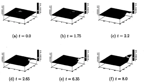
Neumann boundary condition and $R^{2}=0.35$

.

An initial

velocity is imparted to the bubble. In this case, it approaches the boundary of $\Omega$.

After touching the boundary, the bubble

moves

along the boundary. The

more

the

bubble leans against the boundary, the smaller the

area

ofthe surface of the bubble

becomes. Thebubble stops and keeps the smallestsurfacewhen reachingthe corner of

$\Omega$.

(a) $t=0.\mathrm{O}$ (b) $t=1.75$ (c) $t=2.2$

(d) $t=2.65$ (e) $t=6.35$ (f) $t=8.0$

Figure 1: Neumann boundary condition. The bubble which has

an

initial velocity

chosen in such away that it

moves

diagonally,

moves

toward the boundary. After

4.2

Collision of

two

bubbles

The second example treats a collision oftwo bubbleswith the same volume.

After

the collision, thebubbles

merge

and keepthe smallest surface

near

the center of initial

position oftwo bubbles.

$(\mathrm{a})t=0.\mathrm{O}$ $(\mathrm{b})t=0.8$ $(\mathrm{c})t=0.9$

(d) $t=1.1$ (e) $t=1.2$ (f) $t=1.5$

Figure 2: collision of

two

bubbles. Two bubbles separated initially merge into each

other.

4.3

Division

of

oil

droplet

In the third example, the motion of oildrople on the

flat

plane

on

which thereis

a

nonuniform distribution of$\mathrm{s}\mathrm{u}\mathrm{r}\mathrm{f}\mathrm{a}\mathrm{c}\triangleright \mathrm{a}\mathrm{c}\mathrm{t}\mathrm{i}\mathrm{v}\mathrm{e}$

agent is considered.

Thecontact anglebetween the oildropletandtheplaneisprescribed by the affinity

ofthe material of the water surface to the oil droplet surface. Therefore, if there is

a

nonuniform distribution of surface-active agent,

we

can observe that the oil droplet

moves on

the plane driven by the force ofnon-uniformity of the contact angle. The

free-boundary condition

$|\nabla u|^{2}-(u_{t})^{2}=R^{2}$

on

$\partial\{v>0\}$ , (4.1)

which is

obtained

by passing

to

the

limit

as

$\mathit{6}arrow 0$ in (1.1) tells

us

that

we

can

rule

the contact angle of the oil droplet and the plane by defining the coefficient $R$. The

(a) $t=0.0$ (b) $t=0.85$ (c) $t=1.0$

(d) $t=1.15$ (e) $t=1.2$ (f) $t=1.5$

Figure 3: Division of bubble (case 2).

aiming at the part of$\Omega$ withsmaller $R^{2}$. We set

$R^{2}=\{$

0.35

$(x_{1}x_{2}(x_{1}^{2}-x_{2}^{2})\leq 0)$

3.5

otherwise.

4.4

Combination

with

reaction-diffusion equation

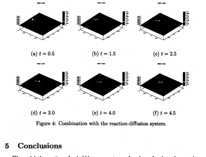
In [11] it is reportedthat

an

oildroplet

on

theglass planeimmersedinsurface-active

agentsolutionimmediately

moves

accordingtothegradient ofthe concentrationofthe

surface-active agent. We

are

trying to realize the motion of the oil droplet numerically

by applying the model of the bubble (1.1) to this phenomenon and combiming it with

reaction-diffusion

equation which shows the time development ofthe concentration of

surface-aetiveagent. Let$v$be the concentrationof surface-activeagent, thenour model

equation of$v$ is

as

follows:

$R^{2}=( \frac{Q}{T})^{2}+\frac{\gamma_{w}(v)-\gamma_{b}}{T}$,

$v_{t}=\kappa\Delta v+\mu(v_{0}-v)v\chi_{u\leq 0}-\nu v\chi_{u>0}$,

$\gamma_{w}=\frac{\gamma_{0}}{1+\alpha v^{\beta}}$

.

Here$T$is the tensionof the oil droplet surface, $\gamma_{w}$ is thetension of glass plane surface

surface have

come

in contact, $Q>0$ is adhesion between the oil and the surface

of plane. In the numerical experiment

we

set

a

$=1,$ $\beta=2$ and impose Neumann

boundary condition. We choose

the

uniform distribution

as

the initial condition

for

$v$.

We

use

the explicit method to solvethis equation. It is observed that the oil droplet

put

near

the boundary

starts

moving aiming at the

area

where the concentration of

the surface-active agent is high. However, the droplet slows down and stops before

reaching the center of the domain, although it should keep moving

as

the experiment

shows. We think that it is nec\’esary to improve the model,

e.g.

by considering the

internal energy of the oil in addition to thesurface energy.

$(\mathrm{a})t=0.5$ $(\mathrm{b})t=1.5$ $(\mathrm{c})t=2.5$

(d) $t=3.0$ (e) $t=4.0$ (f) $t=4.5$

Figure

4:

Combination with the

reaction-diffusion

system.

5

Conclusions

We model the motion of

a

bubble

on

a water

surface by

a

free-boundary

prob-lem with volume conservation constraint and

we

have established

a

numerical method for its solution. The bubble

moves

on

the

water

surfaee

while changing its shape

but preserving its volume. The model equation becomes free-boundary problem of

degenerate hyperbolic type which is difficult to

treat.

We have introduced the time.

semidiscretized variational method to solve this problem and it gives good numerical

results. Thismodel

can

alsobe appliedto themotionof oilon the bottom of water

or to

thiswork hasmanyapplications and is significant for thefuture studying ofhyperbolic

free-boundary problems.

References

[1] H.

W.

Alt- L.

A.

Caffarelli, “Existence and $regula7^{\cdot}ity$

for

a minimum prvblem

with

_free

boundary“, J. Reine Angew. Math., 325 (1981),

105-144.

[2] H. Berestycki - L. A.

Cafafrelli

- L. Nirenberg,

“Uniform

estimates

for

regular-ization

_of

_ffoe

boundaryproblems“, in Analysis and Partial Differential Equation,

Marcel Dekker, NewYork,

1990.

[3] M. Giaquinta, “Multiple integmb in the calculus

_of

variations and nonlinear

el-liptic systems”, Princeton University Press,

1983.

[4] H. Imai - K. Kikuchi - K. Nakane - S. Omata- T. Tachxikawa, $‘ {}^{t}A$ numerical

approach to the asymptotic behavior

_of

solutions

_of

a

one-dimensional hyperbolic

ffee

$bounda\eta$ prvblem“,

JJIAM

18 No.1(2001),

43-58.

[5] K. Kikuchi-S. Omata, $u_{Affee}$ boundary problem

for

a

one

dimensional$h_{\Psi}erbolic$

equation”, Adv. Math.

Sci.

Appl. 9 No.2 (1999),

775-786.

[6]

O.

Ladyzhenskaya- N. Uraltseva, ttLinear and Quasilinear Elliptic Equations”,

Academic

Press, New York and London, 1968.

[7] T. Nagasawa-K. Nakane-

S.

Omata, “Nume$r\dot{\tau}cal$ Computations

for

motion

of

vortioes govemed by

a

Hyperbolic Ginzburg-Landau System”, Nonlinear Anal. 51

(2002) No.1

Ser

A: Theory Methods,

67-77.

[8]

S.

Omata, $‘ {}^{t}A$ Numerical

treatment

of

film

motion utth

_ffee

boundary“,Adv. Math.

Sci. Appl., 14, (2004),

129-137.

[9] T. Yamazaki - S. Omata- H. Yoshiuchi - K. Ohara, $‘ {}^{t}Bubble$ motion

on

water

surface”, Gakuto Intern. Ser. Math.

Sci.

Appl. 23 (2005),

209-216.

[10] T. Yamazaki-S. Omata-K. Svadlcnka-K. Ohara, “Construction

_of

approxi-mate solution to ahyperbolic

_ffee

boundary prvblem utthvolume constraintand its

nume

rical computation“,

Intem.

Ser. Math. Sci.

Appl.

23

(2005),

209-216.

Adv. Math.

Sci.

Appl. 16 No.1 (2006),

57-67.

[11] Y. Sumino-N. Magome-T. Hamada-K. Yoshikawa, “Self-Running $\mathrm{D}\mathrm{r}\mathrm{o}\mathrm{p}\mathrm{l}\mathrm{e}\mathrm{t}+$

Emergence ofRegular Motion fromNonequilibrium Noise”, Phys. Rev. Lett., 94,