The effects of investment lags on the timing of investment and default (Financial Modeling and Analysis)
11
0
0
全文
(2) 2 Because of the investment lags and running costs, the firm can choose to default even before. the project is completed. However, we show that the probability of default in the presence of time‐to‐build is lower than that without time‐to‐build in most cases. The probability of default. before the project’s completion increases in the size of the lags, while that after the completion decreases with time‐to‐build, and the sum of them remains lower than that without time‐to‐build unless it takes an extreme amount of time. This is because the firm makes more conservative. investment and financing decisions as the project takes more time‐to‐build. We also show that the default probability before the project’s completion increases with the project’s profitability. This is because equity holders take more risks for more profitable projects, and Tesla’s recent crisis can be read from this perspective. It made aggressive investment to preempt the mass market of electric cars, but the production lags were much longer than it expected, resulting in. a higher probability of default before any net profits could be made. The remainder of this paper is organized as follows. We describe the setup of the model in Section 2.1 and solve the case of an unlevered firm as a benchmark in Section 2.2. The levered. firm’s choices of investment and financing are investigated in Section 2.3. Section 3 presents and discusses the results of the comparative statics. Section 4 summarizes the main arguments of the paper and discusses future works.. 2. Models and solutions. 2.1. Setup. Suppose that a firm makes the revenue flow Q_{0}X_{t} with a constant Q_{0} and a demand shock X_{t} given by a geometric Brownian motion:. dX_{t}=\mu X_{t}dt+\sigma X_{t}dW_{t} , where. \mu. and. \sigma. (2.1). are positive constants and (W_{t})_{t\geq 0} is a standard Brownian motion on a filtered. space (\Omega, \mathcal{F}, \mathbb{F} :=(\mathcal{F}_{t})_{t\geq 0}, \mathbb{P}) . The risk‐free rate is given by a constant r(>\mu) . The firm can invest in a project to raise the revenue flow to Q_{1}X_{t} , where Q_{1}>Q_{0} , but it takes exponential. time with a parameter. \lambda. to finish the project and raise extra revenue from it. For simplicity,. we assume that the lags are independent of the demand shock. The investment incurs not only lump‐sum costs. I. at the outset of the project but also running costs. i. while the project is in. progress. The firm can issue debt to finance the investment costs and the tax rate is given by. \tau\in[0,1] . For simplicity, we assume a consol bond with a coupon c . Shareholders can choose to default before or after the project is completed, and the firm loses the proportion \alpha\in[0,1] of its value when liquidated. 2.2. Unlevered flrm. As a benchmark, we first examine the case of an unlevered firm. Suppose that the firm has invested in the project and it has been completed. The firm makes the revenue flow Q_{1}X_{t} , and.
(3) 3 the firm value after the completion of the project, V_{1}^{u}(x) , is evaluated as follows:. \Pi_{1}(x) :=E_{t}^{x}[\int_{t}^{\infty}e^{-r(s-t)}(1-\tau)Q_{1}X_{s}ds]=\frac {(1-\tau)Q_{1}x}{r-\mu} .. (2.2). Now, let us suppose that the project has not yet finished. Despite the lump‐sum costs. I. incurred at the outset of the project, the firm makes the revenue flow Q_{0}X_{t} until the project is completed, and running costs. i. are incurred while the project is in progress. Because of these. running costs, shareholders can choose to abandon the ongoing project before its completion. Denoting the timing of the project’s completion and that of abandonment by. T. and T_{a}^{u} , respec‐. tively, the unlevered firm’s value waiting for the completion of the project is. V_{0}^{u}(x)= \sup_{T_{\alpha}^{u} E_{t}^{x}[1_{\{T_{a}^{u}<T\}}\int_{t}^{T_{a} ^{u} e^{-r(s-t)}\{(1-\tau)Q_{0}X_{s}-i\}ds +1_{\{T\leq T_{a}^{u}\} \{\int_{t}^{T}e^{-r(s-t)}\{(1-\tau)Q_{0}X_{s}-i\}ds+e^ {-r(T-t)}V_{1}^{u}(X_{T})\}]. .. (2.3). Before the investment, the firm makes the revenue flow Q_{0}X_{t} and has the option to invest in. the project. Shareholders choose the timing of investment T_{i}^{u} to maximize the firm value, and the firm’s pre‐investment value is. V_{pre}^{u}(x)= \sup_{T_{i}^{u} E_{t}^{x}[\int_{t}^{T_{i}^{u} e^{-r(s-t)}(1- \tau)Q_{0}X_{s}ds+e^{-r(T_{\dot{i} ^{u}-t)}\{V_{0}^{u}(X_{T_{i}^{u} )-I\}]. .. (2.4). From the standard argument of real options theory, the unlevered firm’s optimal investment and abandonment decisions are obtained as follows.. Proposition 1 (Unlevered firm) The optimal investment and abandonment decisions of an all‐equity firm that has an option to invest in a project with time‐to‐build are characterized by the threshold strategies T_{i}^{u*} := \inf\{t>0|X_{t}\geq X_{i}^{u}\} and T_{a}^{u*} := \inf\{t\in[T_{i}^{u*}, T]|X_{t}\leq X_{a}^{u}\}, where the abandonment threshold is. X^{u}= \frac{\gam a_{\lambda}(r+\lambda-\mu)i}{(\gam a_{\lambda}-1)(1-\tau) (Q_{0}+\frac{\lambda}{r-\mu}Q_{1})(r+\lambda)}. (2.5). and the investment threshold is implicitly obtained from. \frac{(\beta-1)(1-\tau)(Q_{1}-Q_{0})\lambda X_{i}^{u} {(r-\mu)(r+\lambda-\mu)} =\frac{(\beta-\gamma_{\lambda})i}{(\gamma_{\lambda}-1)(r+\lambda)}(\frac{X_{i} ^{u} {X_{a}^{u} )^{\gamma_{\lambda} +\beta(\frac{i}{r+\lambda}+I). (2.6). with. \beta=\frac{1}{2}-\frac{\mu}{\sigma^{2} +\sqrt{(\frac{1}{2}-\frac{\mu}{\sigma^ {2} )^{2}+\frac{2r}{\sigma^{2} >1, \gamma_{\lambda}=\frac{1}{2}-\frac{\mu}{\sigma^{2} -\sqrt{(\frac{1}{2}- \frac{\mu}{\sigma^{2} )^{2}+\frac{2(r+\lambda)}{\sigma^{2} <0 .. (2.7). PROOF See Jeon (2018). Given the results in Proposition 1, the unlevered firm’s post‐investment value in (2.3) can be evaluated as follows:. V_{0}^{u}(x)=\Pi_{0}(x)-\Pi_{0}(X_{a}^{u})\Phi_{u}(x) ,. (2.8).
(4) 4 where. \Pi_{0}(x):=(1-\tau)(\frac{Q_{1} {r-\mu}-\frac{Q_{1}-Q_{0} {r+\lambda-\mu})x- \frac{\dot{i} {r+\lambda}. (2.9). is the expected after‐tax revenue before the project’s completion in the absence of default and. \Phi_{u}(x) :=(\frac{x}{X_{a}^{u} )^{\gamma_{\lambda}. (2.10). denotes the state price of the unlevered firm’s abandonment of the project. The derivation of. (2.8) is given in Jeon (2018). Likewise, the unlevered firm’s pre‐investment value in (2.4) can be expressed as follows:. V_{pre}^{u}(x)= \frac{(1-\tau)Q_{0^{X} }{r-\mu}+\{V_{0}^{u}(X_{i}^{u})-\frac{(1 -\tau)Q_{0}X_{i}^{u} {r-\mu}-I\}(\frac{x}{X_{i}^{u} )^{\beta} 2.3. (2.11). Levered firm. We now proceed to the case of a levered firm. The firm can issue debt to finance the investment costs. I. and i , and there is a trade‐off between the tax shields and liquidation costs given the. default.. Suppose that the levered firm’s project has been completed (i.e., t\geq T ). Equity holders choose the timing of default T_{d1} to maximize the equity value:. E_{1}(x)= \sup_{T_{d1}}E_{t}^{x}[\int_{t}^{T_{d1}}e^{-r(s-t)}(1-\tau)(Q_{1} X_{s}-c)ds]. .. (2.12). Given the default decision, the debt value after the project’s completion is. D_{1}(x)= \mathbb{E}_{t}^{x}[\int_{t}^{T_{d1}}e^{-r(s-t)}cds+e^{-r(T_{d1}-t)}(1 -\alpha)V_{1}^{u}(X_{T_{d1}})]. .. (2.13). The firm value after the completion of the project, V_{1}(x) , is the sum of (2.12) and (2.13). Now, let us suppose that the firm has invested in the project but it has not been finished. yet (i.e.,. t<T ).. Equity holders choose the default timing T_{d0} to maximize the equity value:. E_{0}(x)= \sup_{T_{d0}}E_{t}^{x}[1_{\{T_{d0}<T\}}\int_{t}^{T_{d0}}e^{-r(s-t)}\{ (1-\tau)(Q_{0}X_{s}-c)-i\}ds +1_{\{T\leq T_{d0}\} [ \int_{t}^{T}e^{-r(s-t)}\{(1-\tau)(Q_{0}X_{s}-c)-i\}ds+e^ {-r(T-t)}E_{1}(X_{T})]. .. (2.14). The first row of (2.14) corresponds to the expected profits from the case in which the firm defaults before the project is finished (i.e., T_{d0} ), while the second row represents the expected profits from the case in which the firm defaults after the project is completed (i.e., T_{d1} ). Given these default decisions, the debt value before the project’s completion is. D_{0}(x)= E_{t}^{x}[1_{\{T_{d0}<T\}}\{\int_{t}^{T_{d0}}e^{-r(s-t)}cds+e^{- r(T_{d0}-t)}(1-\alpha)V_{0}^{u}(X_{T_{d0}})\}+1_{\{T\leq T_{d0}\} D_{1}(x)] . (2.15) The value of the levered firm waiting for the completion of the project, V_{0}(x) , is the sum of. (2.14) and (2.15)..
(5) 5 Shareholders choose the timing of investment T_{i} and amount of debt financing. c. to maximize. the pre‐investment firm value:. V_{pre}(x)= \sup_{T_{\dot{i} ,c}E_{t}^{x}[\int_{t}^{T_{i} e^{-r(s-t)}(1-\tau)Q_ {0}X_{s}ds+e^{-r(T_{i}-t)}\{V_{0}(X_{T_{i} )-I\}]. .. (2.16). Given these arguments, we can derive the levered firm’s optimal investment, default, and financing decisions as follows.. Proposition 2 (Levered firm) The optimal investment, default, and financing decisions of a firm that has an option to invest in a project with debt financing in the presence of time‐to‐ build are characterized by the thresholds strategies T_{i}^{*} := \inf\{t>0|X_{t}\geq X_{i}\}, T_{d0}^{*} := \inf\{t\in. [T_{i}^{*}, T]|X_{t}\leq X_{d0}\} , and T_{d1}^{*} := \inf\{t>T|X_{t}\leq X_{d1}\} , where the thresholds of investment and default and the coupon payment are obtained as the solutions of the following system of equations:. X_{i}= \frac{(r+\lambda-\mu)(r-\mu)}{(\beta-1)(1-\tau)(Q_{1}-Q_{0})\lambda} [\{\alpha\Pi_{0}(X_{d0})+(1-\alpha)\Pi_{0}(X_{a}^{u})+\frac{\tau c}{r}\}(\beta- \gamma_{\lambda})\Phi_{0}(X_{i}) + \{\alpha\Pi_{1}(X_{d1})+\frac{\tau c}{r}\}\{(\beta-\gamma_{\lambda})\Phi_{1} (X_{i})+(\gamma_{\lambda}-\gamma)(\frac{X_{i} {X_{d1} )^{\gamma}\}+ \beta(\frac{i}{r+\lambda}-\frac{\tau c}{r}+I)],. X_{d0}=\frac{r+\lambda-\mu}{(1-\gam a_{\lambda})(Q_{0}+\frac{\lambda}{r-\mu}Q_ {1}) [\frac{(\gam a_{\lambda}-\gam a)c}{(1-\gam a)r}(\frac{X_{d0} {X_{d1} ) ^{\gam a}-\gam a_{\lambda}(\frac{ }{r}+\frac{i}{(1-\tau)(r+\lambda)} ]. ,. (2.17) (2.18). X_{d1}= \frac{\gamma(r-\mu)c}{(\gamma-1)rQ_{1} ,. (2.19). c=\frac{rX_{d0}{\gam a_{\lambda}-\frac{\gam a_{\lambda}-\gam a}{1-\gam a} (h\frac{X_{d0}{X_{d1})^{\gam a}[\frac{\alpha(1-\tau)(1-\gam a_{\lambda}) (Q_{0}+\frac{\lambda}{r-\mu}Q_{1}){(r+\lambda-\mu)\tau}+ \frac{\alpha\gam a_{\lambda^{\dot{i} {(r+\lambda)\tauX_{d0}-\frac{1-\Phi_{0} (X_{i})-h^{\gam a}\Phi_{1}(X_{i}){r\psi\Phi_{0}(X_{i})] (2.20). with. \gamma=\frac{1}{2}-\frac{\mu}{\sigma^{2} -\sqrt{(\frac{1}{2}-\frac{\mu} {\sigma^{2} )^{2}+\frac{2r}{\sigma^{2} <0 ,. \psi=\frac{r-\mu}{r[\frac{\gam a_{\lambda}+(\gam a-\gam a_{\lambda})(\frac{X_ {d0}{X_d1})^{\gam a}{\frac{\gam a_{\lambda}-1{r+\lambda-\mu}\{(r-\mu)Q_{0}+ \lambdaQ_{1}\+(\gam a-\gam a_{\lambda})Q_{1}(\frac{X_d0}{X_d1})^{\gam a-1} ] h=(1- \gamma-\frac{\alpha(1-\tau)\gamma}{\tau})^{-\frac{1}{\gamma}. (2.21) ,. (2.22) (2.23). PROOF See Jeon (2018).. Given the results in Proposition 2, the equity and debt values in (2.14) and (2.15) can be expressed as follows:. E_{0}(x)= \Pi_{0}(x)-\frac{(1-\tau)c}{r}-\{\Pi_{0}(X_{d0})-\frac{(1-\tau)c}{r} \}\Phi_{0}(x)-\{\Pi_{1}(X_{d1})-\frac{(1-\tau)c}{r}\}\Phi_{1}(x). ,. (2.24). D_{0}(x)= \frac{c}{r}-\{\frac{c}{r}-(1-\alpha)V_{0}^{u}(X_{d0})\}\Phi_{0}(x)-\{ \frac{c}{r}-(1-\alpha)V_{1}^{u}(X_{d1})\}\Phi_{1}(x) ,. (2.25).
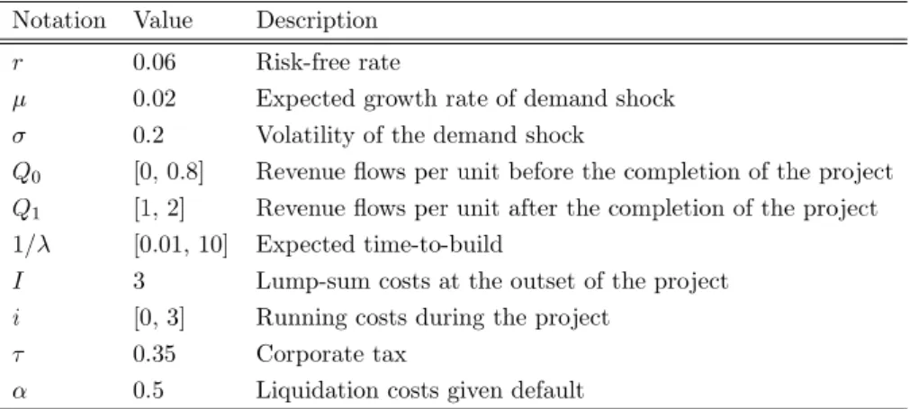
(6) 6 where. \Phi_{0}(x)=(\frac{x}{X_{d0} )^{\gamma_{\lambda} \Phi_{1}(x)=(\frac{x}{X_{d1} })^{\gamma}-(\frac{x}{X_{d0} )^{\gamma_{\lambda} (\frac{X_{d0} {X_{d1} ) ^{\gamma}. (2.26). denote the state prices of the levered firm’s default before and after the completion of the project, respectively. The firm value is the sum of equity and debt values:. V_{0}(x)= \Pi_{0}(x)+\frac{\tau c}{r}-\{\alpha\Pi_{0}(X_{d0})+(1-\alpha)\Pi_{0} (X_{a}^{u})(\frac{X_{d0}}{X_{a}^{u} )^{\gamma_{\lambda} +\frac{\tau c}{r}\}\Phi_ {0}(x)-\{\alpha\Pi_{1}(X_{d1})+\frac{\tau c}{r}\}(2.27) \Phi_{1}(x). .. It is straightforward that the equity, debt, and firm values after the project’s completion are evaluated as follows:. E_{1}(x)= \Pi_{1}(x)-\frac{(1-\tau)c}{r}-\{\Pi_{1}(X_{d1})-\frac{(1-\tau)c}{r} \}(\frac{x}{X_{d1}})^{\gamma}. D_{1}(x)= \frac{c}{r}-\{\frac{c}{r}-(1-\alpha)\Pi_{1}(X_{d1})\}(\frac{x}{X_{d1} })^{\gamma} V_{1}(x)= \Pi_{1}(x)+\frac{\tau c}{r}-\{\alpha\Pi_{1}(X_{d1})+\frac{\tau c}{r} \}(\frac{x}{X_{d1}})^{\gamma}. (2.28) (2.29) (2.30). Lastly, the levered firm’s pre‐investment value in (2.16) can be rewritten as follows:. V_{pre}(x)= \frac{(1-\tau)Q_{0^{X} }{r-\mu}+\{V_{0}(X_{i})-\frac{(1-\tau)Q_{0} X_{i} {r-\mu}-I\}(\frac{x}{X_{\dot{i} })^{\beta} 3. (2.31). Comparative statics and discussion. To allow a comparison, we use a benchmark model without time‐to‐build (e.g., Sundaresan et al.. (2015)). To denote the values associated with the benchmark model, we use a bar on the top of each value. For the numerical calculation, we use the following parameters: Notation. V a1ueDescr\dot{{\imath}} ption. \overline{\overline{r0.06Risk-freerate}} \mu. 0.02. Expected growth rate of demand shock. \sigma. 0.2. Volatility of the demand shock Revenue flows per unit before the completion of the project. 1/\lambda. [0,0.8] [1, 2] [0.01, 10]. I. 3. Lump‐sum costs at the outset of the project. Q_{0} Q_{1}. i. [0,3]. Revenue flows per unit after the completion of the project Expected time‐to‐build Running costs during the project. \tau. 0.35. Corporate tax. \alpha. 0.5. Liquidation costs given default Table 1: Parameters for the numerical calculation.
(7) 7. 1. 2. 3. 4. 5. 6. 7. 8. 9. 10. 1. 2. 3. 4. 5. 6. 7. 8. 9. 10. 1/\lambda 1/\lambda. (a) Optimal investment thresholds. (b) Optimal default/abandonment thresholds 0. 0. 0. 0. 0. 0 1. 2. 3. 4. 5. 6. 7. 8. 9. 10. 1. 2. 3. 4. 5. 6. 7. 8. 9. 10. 9. 10. 1/\lambda 1/\lambda. (c) Optimal coupon payment. (d) Optimal leverage ratios. 0. 0. 0. 0 0. 0. 0. 0. 0 1. 2. 3. 4. 5. 6. 7. 8. 9. 10. 1. 2. 3. 4. 5. 6. 7. 8. 1/\lambda 1/\lambda. (e) State prices of default/abandonment. (f) State prices of default. Figure 1: Comparative statics with respect to the expected time‐to‐build Figure 1 presents the results of the comparative statics with regard to expected time‐to‐. build (i.e., 1/\lambda). Figure la shows that the investment is delayed when it requires time‐to‐build, irrespective of its financing method (i.e., X_{i}>\overline{X}_{i} and X_{i}^{u}>\overline{X}_{i}^{u} ) and that the delay becomes.
(8) 8 significant as expected time‐to‐build becomes longer. This is a natural result because the project. becomes less profitable as it takes more time to yield revenue, in line with Weeds (2002) and Alvarez and Keppo (2002). The former study examined firms’ R&D competition with an un‐ certain discovery time and showed that such investment can be delayed despite the presence of preemption incentives. The latter elaborated on uncertainty in the lags by assuming that they. depend on the underlying revenue process and showed that the investment is delayed signifi‐ cantly. These works, however, were limited to the analysis of unlevered firms, lacking discussions of financing decisions.. Figure lb shows that the default thresholds in the presence of time‐to‐build are higher than. those in the absence of time‐to‐build (i.e., X_{d0}, X_{d1}>\overline{X}_{d} ) and that they strictly increase in the size of investment lags. This, however, does not imply that the default probability is an increasing function of time‐to‐build, as discussed shortly. We can also see that the threshold of. default before the project’s completion is higher than that after completion (i.e., X_{d0}>X_{d1} ). This is a natural result because the firm incurs running costs and raises less revenue before the project is completed.. Regarding the amount of debt financing, Figure lc shows that the coupon payment optimally. chosen by equity holders is higher when the project requires time‐to‐build (i.e.,. c>\overline{c} ). and that. it strictly increases as the expected lags become longer. This is because the firm expects more running costs as the lags increase, which makes it depend more on debt to finance the investment costs.. The leverage ratio, however, is not monotone with respect to the size of investment lags. Figure ld shows that the optimal leverage ratio is inverted. U ‐shaped. with respect to 1/\lambda . When. expected time‐to‐build is not significant, the firm raises the leverage ratio as it takes more. time to complete the project. After the lags exceed a certain level (approximately two years with the benchmark parameters), it starts to lower the leverage ratio as time‐to‐build increases because of the concern about default before the project’s completion. This inverted. U ‐shaped. leverage ratio is consistent with the findings of Agliardi and Koussis (2013), who studied the impact of time‐to‐build with a dynamic debt structure. Their model, however, postulated that the investment timing is exogenously given and that there is no uncertainty in time‐to‐build, whereas the investment timing is endogenously determined with uncertainty in time‐to‐build in. our model. Despite the inverted. U ‐shape,. the leverage ratio with time‐to‐build is found to be. higher than that without time‐to‐build.. These results, however, do not imply that the presence of time‐to‐build always raises the probability of default. Figure le presents the state price of default before and after the project’s. completion at the timing of investment, which is directly linked to the default probability. As the investment lags become longer, the probability of default before the project’s completion strictly increases, whereas that after the project’s completion strictly decreases. The sum of them is given in Figure lf, which shows that the default probability in the presence of time‐to‐build is. U ‐shaped. and lower than that without lags unless it takes an extreme amount of time (more than seven years with the benchmark parameters). This finding implies that the firm makes conservative investment and financing decisions when the investment involves uncertain time‐to‐build. Note.
(9) 9 that the investment trigger strictly increases in the size of lags and the leverage ratio does not monotonically increase in the expected time‐to‐build in spite of increasing expected running costs.. 1. 31. 3 1. 31 1. 3. 1. 31. 3 1. 31 1. 3. 31 02. 04. 06. 08. 1. 12. 14. 1 6. 18. 02. 04. 06. 08. 1. 1 2. 14. 1 6. 18. 1/\lambda 1/\lambda. (a) Optimal investment thresholds when. c=3. 4. (b) Optimal investment thresholds when. c=5. 55. 5 43 55 4. 5. 55. 43. 5 4. 55. 43. 5 02 04 06 08 1 12 14 1 6 18 02 04 06 08 1 1 2 14 1 6 18. 1/\lambda 1/\lambda. (c) Optimal investment thresholds when. c=7. (d) Optimal investment thresholds when. c=9. Figure 2: Comparative statics with respect to the expected time‐to‐build given exogenous coupon payment. The results in Figures la showed that the timing of investment is delayed under time‐to‐. build (i.e., X_{i}>\overline{X}_{i} ). These results are based on the optimal capital structure that maximizes the firm value, given in Proposition 2, and they do not hold when the firm is not optimally levered. Figure 2 shows that when the firm is highly levered, the investment triggers are concave with respect to expected time‐to‐build and can be even lower than that without investment lags.. In other words, equity holders have an incentive to accelerate the investment at the expense of debt holders.. Bar‐Ilan and Strange (1996) also showed that a firm can hasten the investment in the presence of lags, suggesting that the lags lower the value of option to wait. Their model, however, assumed no uncertainty in the lags and did not consider debt financing, leaving the question of how time‐ to‐build affects the financing decision unanswered. To be more specific, their work studied an.
(10) 10 all‐equity firm’s investment with fixed lags and there is no running cost while the project is. in progress. Since the abandonment of the ongoing project incurs nonnegative costs, the firm always waits until the project is finished. By contrast, our model incorporates debt financing and. uncertainty in the lags with running costs, and the equity holders can choose to default before the project is completed. In this framework, we show that the conflicts of interest between equity and debt holders can accelerate the investment despite uncertainty in time‐to‐build. To our best. knowledge, our study is the first to investigate the risk‐shifting in the presence of time‐to‐build.. Sarkar and Zhang (2015) studied two‐stage investment with implementation lags and debt financing, showing that the investment triggers are inverted. U ‐shaped. when the firm is highly. levered. In their model, however, the triggers are decreasing functions of the lag when the firm’s debt level is low or it is optimally levered. The difference comes from the description of the investment lags. They described the lag by the lumpiness of the investment, assuming that the trigger of second‐stage investment is proportional to that of the first‐stage one, whereas we directly model time‐to‐build with uncertainty.. 4. Conclusion. In this study, we derived a firm’s optimal investment, financing, and default choices in the presence of time‐to‐build. We showed that a firm that makes an optimal financing decision delays investment because of these investment lags, whereas a highly levered firm rather hastens such investment. Because of the running costs incurred during the lags, the firm can choose to default before the project is completed. Nonetheless, the probability of default with time‐to‐build is lower than that without time‐to‐build in most cases. The optimal leverage ratio is found to be. inverted. U ‐shaped. with respect to the size of the lags. As the project becomes more profitable,. the firm invests more aggressively, which leads to an increase in the default probability before completion.. A range of problems remain to be tackled. For instance, we analyzed a representative firm’s investment and financing decisions in the presence of time‐to‐build; however, market competition might dramatically change the results. Owing to the incentive to preempt the market, even an optimally levered firm might choose to accelerate the investment despite uncertainty in time‐to‐ build. Furthermore, asymmetric information between competitors regarding each other’s time‐ to‐build might yield strategic interactions between them. For the extension of financing methods, one can consider external financing constraints, which are likely to be imposed on the firm with a project that requires time‐to‐build. The effects of debt restructuring in the presence of time‐ to‐build remain to be studied as well. It is to be hoped that our study will serve as a platform to research these issues further.. References. Agliardi, E. and Koussis, N. (2013), ‘Optimal capital structure and the impact of time‐to‐build’, Finance Research Letters 10, 124‐130..
(11) 11 11 Alvarez, L. and Keppo, J. (2002), ‘The impact of delivery lags on irreversible investment under uncertainty’, European Journal of Operational Research 136, 173‐180.. Bar‐Ilan, A. and Strange, W. (1996), ‘Investment lags’, American Economic Review S6, 610‐622. Jeon, H. (2018), Investment and financing decisions in the presence of time‐to‐build. Working paper.. Sarkar, S. and Zhang, C. (2015), ‘Investment policy with time‐to‐build’, Journal of Banking and Finance 55, 142‐156.. Sundaresan, S., Wang, N. and Yang, J. (2015), ‘Dynamic investment, capital structure, and debt overhang’, Review of Corporate Finance Studies 4, 1‐42.. Weeds, H. (2002), ‘Strategic delay in a real options model of R&D competition’, Review of Economic Studies 69, 729‐747.. Center for Mathematical Modeling and Data Science Osaka University, Toyonaka 560‐0043, Japan E‐mail address: [email protected]‐u.ac.jp.
(12)
図

関連したドキュメント
Standard domino tableaux have already been considered by many authors [33], [6], [34], [8], [1], but, to the best of our knowledge, the expression of the
The relevant difference between the two kinds is that uninformed agents base their investment decision through an imitative behavior also called herding while informed ones follow
Many authors argue that as the investment horizon increases, an investment portfolio with a higher proportion of assets will dominate, or will be preferred over a portfolio
Which decisions about the depos- itory consumption, value of the investment in loans, and provisions for loan losses must be made in order to maximize banking profit on a random
Let us consider a switch option, the payoff of which at maturity is set to equal the value at that time of an investment project with possible entry and exit.. The underlying
Let us consider a switch option, the payoff of which at maturity is set to equal the value at that time of an investment project with possible entry and exit.. The underlying
Eskandani, “Stability of a mixed additive and cubic functional equation in quasi- Banach spaces,” Journal of Mathematical Analysis and Applications, vol.. Eshaghi Gordji, “Stability
We investigated a financial system that describes the development of interest rate, investment demand and price index. By performing computations on focus quantities using the
