より効率的なフィルタリング型ブースティング技法(計算理論とアルゴリズムの新展開)

より効率的なフィルタリング型ブースティング技法

An Efficient Smooth Boosting

by

Filtering

畑町晃平

\dagger

Kohei

Hatano

九州大学システム情報科学研究院情報理学部門

DepartmentofInformatics, KyushuUniversity

Abstract

Boosting is ageneral method to construct a highly accurate classifier by combining “weakly”

ac-curate ones. Smooth boosting algorithmsarevariants ofboostingmethods which handleonlysmooth

distributions onthe data. They are proved tobe noise-tolerant and canbe used in the “boosting by

filtering” scheme, which is suitable for learning over huge data. However, current smooth boosting

algorithms have rooms for improvements: A non-smooth boosting algorithm, InfoBoost canperform

moreefficiently thantypicalboosting algorithmns byusinganinformation-theoretic criterion for choosing

hypotheses. In this paper, we propose anewsmooth boosting algorithm withan information-theoretic

criterion andweshow thatitinheritsthe advantages of twoapproaches,smooth boosting andInfoBoost.

1

Introduction

Inrecentyears, huge data havebecome available

due tothe developmentof computers and the

Inter-net. In knowledgediscovery and machine learning

tasks, size of such huge data

can

reach hundreds

ofgigabytes or

more.

So it is important to make

knowledge discoveryormachine learning algorithms

scalable. Sanipling is one ofeffective techniques to

dealwith large data. Thatis, instead of usingwhole

the data, wecan obtain asumniaryofthedata by

sampling randomly from it. There

are

many

re-sults on sampling techniques (see,

e.g.,

[4]) and

applicationsto data mining tasks such

as

decision

tree learning [6], support vector machine [2], and

boosting $[4, 5]$

.

Especially, boosting is simple andefficient

learn-ing method

among

machine learning algorithms.

The basic idea of boosting is combining many

slightly accuratehypotheses(which _{we call “weak”}

hypotheses) into

a

highly accurate

one.

Originally,

boosting

was

invented underthe boosting by

filter-ing framework, where the booster

can

sample

ex-amplesrandomly from

the whole

data [16, $\eta$

.

The

main advantage of the filtering

framework

is

that

2Email: [email protected] jp

the learnerneedto store lessexamples. Ingeneral,

the learner have to store manyexample enough in

ordertoevaluate its finalhypothesis. On the other

hand, in boosting by framework, the booster does

not have to store all sampled examples, but have

to keep examples only for learning weak hypothe

ses, which is much smaller than those forthe final

hypotheses. Sothe boostingbyfilteringfiiamework

seems

tofitlearningtasks

over

huge data. However,

early boosting algorithms [16, $\eta$ which workinthe

filtering

framework

were

not practical because they

were

not adaptive, i.e., they need theprior

knowl-edge

on

the

accuracy of

weak hypotheses.

Madaboost,

a

modification of$\mathrm{A}\mathrm{d}\mathrm{a}\mathrm{B}\mathrm{o}\mathrm{o}\mathrm{s}\mathrm{t}[8]$,is the

firstadaptive boosting algorithmwhich worksinthe

filtering framework [5]. Combining with adaptive

sampling methods [4], Madaboost is shown to be

more

efficient than$\mathrm{A}\mathrm{d}\mathrm{a}\mathrm{B}\mathrm{o}\mathrm{o}\mathrm{e}\mathrm{t}$

over

huge data,while

keeping the prediction accuracy. By its nature of

updating scheme, MadaBoost is categorized

as one

of(ismooth” _{boosting algorithms} $[18, 9]$, where the

name, smooth boosting,

comes

from the fact that

these

boosting algorithms only deal with

smooth

distributions

over

data (In contrast, for example,

dis-tributions

over

data). Smoothness of distributions

enables boosting algorithms to sample data

effi-ciently. Also,smoothboostingalgorithms have

the-oretical guarantees for noise tolerance in the

vari-ousnoisy learning settings,such

as

statisticalquery

model [5], malicious noise model [18] and agnostic

boosting [9].

However

it

seems

that there is still

room

for

im-provements

on smooth

boosting. A non-smooth

boosting algorithm,

InfoBoost

[1] (which is

a

spe-cial form of real $\mathrm{A}\mathrm{d}\mathrm{a}\mathrm{B}\mathrm{o}\mathrm{o}\mathrm{s}\mathrm{t}[17])$, performs

more

efficiently than other boosting algorithms in the

boosting by subsampling framework, where only a

bunch of data isgiven in advance. Moreprecisely,

givenhypotheseswith

error

1/2-7/2$(0<\gamma<1)$,

typical boostingalgorithmstake$O(1/\gamma^{2})$ iterations

to learn sufficiently accurate hypothesis. On the

other hand, InfoBoost learns in from $O(1/\gamma)$ to

$O(1/\gamma^{2})$ iterationsbytaking advantage

of

the

situ-ationwhen weak hypotheses have low

false

positive

error

$[10, 11]$. So InfoBoost

can

be

more

efficient

at most by$O(1/\gamma)$ times.

The main differencebetweenInfoBoost andother

boosting algorithms such as $\mathrm{A}\mathrm{d}\mathrm{a}\mathrm{B}\mathrm{o}\mathrm{o}\mathrm{e}\mathrm{t}$ or Mad-$\mathrm{a}\mathrm{B}\mathrm{o}\mathrm{o}\mathrm{s}\mathrm{t}$ is the criterion for

choosing weakhypothe

ses.

Typical boosting algorithms

are

designed to

choose hypotheseswhose errors are nnnimumwith

respect to given distributions. In contrast,

In-$\mathrm{f}\mathrm{o}\mathrm{B}\mathrm{o}\mathrm{o}\mathrm{s}\mathrm{t}$

uses an

information-theoretic criterion to

choose weak hypotheses. The criterion was

previ-ously proposed by Kearns and

Mansour

[12], and

also applied to boosting algorithms using decision

trees[12] andbranching

programs

[14]. But, sofar,

no

smooth algorithmis known to have such the nice

propertyofInfoBoost.

In this paper, we modify

one

of smooth boost-ing algorithms, $\mathrm{A}\mathrm{d}\mathrm{a}\mathrm{F}\mathrm{l}\mathrm{a}\mathrm{t}[9]$

, as

it is quite similar

to

MadaBoost

and yet simple to analyze.

Our

modification is derived in a similar way that

In-$\mathrm{f}\mathrm{o}\mathrm{B}\mathrm{o}\mathrm{o}\mathrm{s}\mathrm{t}$ is given. As a result,

we

propose a

new

smooth boostimg algorithm with yet another information-theoretic criterion. Our preliminary

experiments show that

our

modification, which

we

call

MadaFlat

(Modification

of

$\mathrm{A}\mathrm{d}\mathrm{a}\mathrm{F}\mathrm{l}\mathrm{a}\mathrm{t}$),

outper-forms MadaBoostinthe filtering framework.

2 Preliminaries

2.1 Learning Model

We adapt the

PAC

learning model [19]. Let $\mathcal{X}$

be

an

instance space andlet$\mathcal{Y}=\{-1, +1\}$beaset

oflabels. We

assume

an

unknown target

_function

$f$: $\mathcal{X}arrow \mathcal{Y}$

.

Furtherwe

assume

that _$f$is contained in

a

known

class

$F$of

functions

from$\mathcal{X}$

to

$\mathcal{Y}$

.

Let$D$

bean unknown

distribution

over

$\mathcal{X}$

.

The learner has

an access

to the example oracle $\mathrm{E}\mathrm{X}(f, D)$

.

When

given

a

call from

the learner, $\mathrm{E}\mathrm{X}(f, D)$ returns

an

example$(x, f(x))$ _{where each}$x$is drawnrandomly

according to $D$

.

Let $\mathcal{H}$ be

a

hypothesis space,

or

a set of functions from X to $\mathcal{Y}$

.

We

assume

that $\mathcal{H}\supset \mathcal{F}$

.

For any distribution _$D$

over

X,

er-ror

ofhypothesis $h\in \mathcal{H}$ is defined as $\mathrm{e}\mathrm{r}\mathrm{r}_{D}(h)\mathrm{d}\mathrm{e}\mathrm{f}=$

$\mathrm{P}\mathrm{r}_{D}\{h(x)\neq f(x)\}$

.

Let $S$ be a sample, a set of

examples $((x_{1}, f(x_{1}),$

$\ldots,$$(x_{m}, f(x_{m})))$

.

For any

sample $S$, training

error of

hypothesis $h\in \mathcal{H}$ is

defined

as

$\overline{\mathrm{e}\mathrm{r}\mathrm{r}}_{S}(h)\mathrm{d}\mathrm{e}\mathrm{f}=|\{(x_{i}, f(x_{i})\in S|h(x_{t})\neq$

$f(x_{i})\}|/|S|$

.

Now

we define PAC

learnability

as

follows.

Deflnition 1 (Strong learning). A learning

al-gorithm $A$ is

a

strong leamerfor _$F$ if and only if,

for any $f\in F$ and any distribution $D$, given $\vee c$, $\delta$

$(0<\epsilon, \delta<1)$,

a

hypothesis space$\mathcal{H}$, and

access

to

the example oracle$\mathrm{E}\mathrm{X}(f, D)$ asinputs,$A$outputsa

hypothesis $h\in \mathcal{H}$ such that$\mathrm{e}\mathrm{r}\mathrm{r}_{D}(h)=\mathrm{P}\mathrm{r}_{D}\{h(x)\neq$

$f(x)\}\leq\epsilon$ with probabilityat least 1–6.

On the otherhand,

an

apparentlyweakernotion

of learningwasproposed [16].

Deflnition2 (Weak learning). Alearning

algo-rithm$A$is

a

weak leanerfor$\mathcal{F}$ifand only if, forany

$f\in F$, given a hypothesis space $\mathcal{H}$, and

access

to

the example oracle $\mathrm{E}\mathrm{X}(f.D)$ as inputs, $A$ outputs

a

hypothesis $h\in \mathcal{H}$ such that

err

_{$D(h)\leq 1/2-\gamma/2$}

for a fixed7 $(0<\gamma<1)$

.

2.2 $\mathrm{B}o$ostingApproai

Schapireprovedthatstrongandweak

PAC

learn-ability

are

equivalent to each other for the

first

a strong learner by using a weak learner is called

“boosting”. Basic idea of boosting is the

follow-ing: First, the booster trains a weak learner with

respect to different distributions $D_{1},$ $\ldots$,$D_{T}$

over

the domain $\mathcal{X}$, and gets different “weak“

hypothe-ses

$h_{1},$

$\ldots$,$h_{T}$ such thaterr$D_{f}(h_{t})\leq 1/2-\gamma_{t}/2$ for

each$t=1,$$\ldots,$$T$

.

Then the booster combines weak

hypotheses$h_{1},$

$\ldots,$$h_{T}$into

a

final hypotheses $h_{final}$

satisfying

err

$D(h_{fina\iota})\leq\epsilon$

.

Definition 3. Let and be any distributions

over

$\mathcal{X}$

.

Wesay that $D’$ is $\lambda$-smooth with respect

to $D$ if$\sup_{X\in \mathcal{X}}D’(x)/D(x)\leq\lambda$_.

The smoothness parameter A has crucial roles in robustness of boosting algorithms [5, 18, 9]. Also,

it affects the efficiency of sampling methods. For

example, byrejection sampling,

we

use

$1/\lambda$calls

of

$EX(f, D)$

on

averageto

simulate

a

call of$\mathrm{E}\mathrm{X}(f, D’)$

for

a

distribution$D’$ that isA-smooth$\mathrm{w}$

.

$\mathrm{r}$

.

$\mathrm{t}$

.

$D$

.

Subsampling

versus

Filtering We consider

two

frameworks

of boosting, boosting by

subsam-pling and boosting by filtering. In the

subsam-pling framework, the booster is given

a

sample

$S=((x_{1}, f(x_{1}),$_$\ldots,$$(x_{m}, f(x_{m})))$ in advance. The

booster constructs thefinal hypothesis whose

train-ing $\overline{\mathrm{e}\mathrm{r}\mathrm{r}}s(h_{f\dot{*}nal})\leq\epsilon$ by training the weak learner

over

the given sample $S$

.

Then the

generaliza-tion

error

is estimatedby using arguments

on

VC-dimensions

or

margin (E.g.,

see

[15]). For

exam-ple, for typical boosting algorithms,$\mathrm{e}\mathrm{r}\mathrm{r}_{D}(h_{f:na1})\leq$

$\overline{\mathrm{e}\mathrm{r}\mathrm{r}}s(h_{f1na\mathrm{t}})+\tilde{O}(\sqrt{T\log|W|}/m)$ 1 with high

prob-ability, where$T$ is the size ofthe final hypotheses,

i.e., the number of weak hypotheses combined in

$h_{f_{t\hslash a\iota}}$

.

In the filtering framework, on the other hand,

the booster deal with the whole instance space $\mathcal{X}$

through $\mathrm{E}\mathrm{X}(f, D)$

.

By using statistics obtained

from calls of $\mathrm{E}\mathrm{X}(f, D)$, the booster tries to mini-mizes

err

$D(h_{fina\iota})$ directly. There

are

two

advan-tages of the boostingbyfilteringover the boosting

by subsampling.

First of

all, the

space

complexity

is reduced. Roughly speaking, the booster needs

tostore$\tilde{O}(T\log|W|)$ examples in the subsampling

framework,whereas,the boosteronly needtostore

$\tilde{O}(\log|\dagger V|)$ examples in the filtering framework.

Second,thebooster does not havetodeterminethe

size of sample $S$ a priori. There advantages are

preferablefor learning

over

huge data.

Smooth Boosting Smooth boosting algorithms only deal such

distributions

$D_{1},$

$\ldots,$$D_{t}$ that

are

“smooth” with respect to the original

distribution

$D$

.

We

define

the following

measure

ofsmoothness.

1Inthe$\overline{O}(.q(n))$ notation,weneglectpoly$(1\mathrm{o}g(n))$terms.

Our Assumption and Technical Goal In the

rest of the paper,

we

assume

the weak hypothesis

assumption

on

$W$

as

follows: The learner isgiven

a

finite set $W$ ofhypothesessuchthat for any

distri-bution$D’$ over X, there existsahypothesis$h\in W$

satisfying$\mathrm{e}\mathrm{r}\mathrm{r}_{D’}(h)\leq 1/2-\gamma/2(0<\gamma<1)$

.

Now our technicalgoalisto construct

an

efficient

smooth boostingalgorithmwhich worksinboth the

subsamplingand

the

filtering

framework.

3 $\mathrm{B}o$ostingby Subsampling

In this section, we propose a modification of

$\mathrm{A}\mathrm{d}\mathrm{a}\mathrm{F}\mathrm{l}\mathrm{a}\mathrm{t}$ inthe subsampling framework. Let

$\ell(x)=\{$

1, $x\geq 0$

$x-10,$’

$x\leq-1-1<x.<0$

The description of

our

modification is given in

Figure 3 Given

a

sample $S=((x_{1}, f(x_{1}))$,

..

.

,

$(x_{m}, f(x_{m})))$, and

a

combined hypothesis $H_{t}=$

$\sum_{j=1}^{t}\alpha_{j}[h_{j}(x)]h_{j}(x)$ at iteration$t$, pseudo gain of hypothesis $h$is given as

follows:

$\Delta_{t}(h)$ $=$ $\frac{m_{h,+}}{m}\mu_{h,t},[+1]^{2}\gamma_{h,t}[+1]^{2}$ $+ \frac{m_{h,-}}{m}\mu_{h,t}[-1]^{2}\gamma_{h,t}[-1]^{2}$

.

where

$\mu_{h,t}[\pm 1]=\frac{1}{m_{h,\pm}}.\sum_{:h(x_{:})=\pm 1}\ell(-f(x:)H_{t}(x.))$,

$\gamma_{h.\ell}[\pm 1]=\frac{\sum_{:.h(X.)=\pm 1}f(x.)h(x:)D_{\mathrm{t}}(i)}{\sum_{i\cdot h(l_{l})=\pm 1}D_{f}(i)}$,

$D,(x_{i})= \frac{\ell(-f(x_{i})H_{t}(x_{i}))}{\sum_{i=1}^{m}\ell(-f(x_{*})H_{t}(x.))}$,

and $m_{h,\pm}=|\{i : h(x_{i})=\pm 1\}|$ (In

the

case

when $m_{h,\pm}$ is zero,

we

assume

that $\mu_{h.t}[\pm 1]=$

$\gamma_{h.t}[\pm 1]=0)$

.

At each iteration $t$,

our

algorithm MadaFlat chooses hypothesis $h$thatmaximizes its

$\mathrm{M}\mathrm{a}\mathrm{d}\mathrm{a}\mathrm{F}\mathrm{l}\mathrm{a}\mathrm{t}_{filt}(\epsilon, \delta, \mathrm{E}\mathrm{X}(f, D))$

begin

l.Let $H_{1}(x)=0;tarrow 1;\delta_{1}arrow\delta/4$;

2. while

_Pt

$\geq\frac{4\ }{5}$ do

a) $(h_{t}, S_{t})arrow \mathrm{H}\mathrm{S}\mathrm{e}\mathrm{l}\mathrm{e}\mathrm{c}\mathrm{t}(1/2,\delta_{t})$;

b) $(\hat{\mu}_{t},\hat{\mu}_{t}[+1],\hat{\mu}_{f}[-1], \gamma_{\ell}[’+1],\hat{\gamma}_{\ell}[-1])$

$arrow \mathrm{e}\mathrm{m}\mathrm{p}\mathrm{i}\mathrm{r}\mathrm{i}\mathrm{c}\mathrm{a}\mathrm{l}$ estimatesover $S_{t}$;

c) at$[+1]arrow\mu_{t}’[+1]’\gamma_{\mathrm{t}}[+1];\alpha_{\mathrm{t}}[-1]arrow\hat{\mu}_{t}[-1]\hat{\gamma}_{\mathrm{t}}[-1]$;

d) $H_{+1},(x)arrow H_{t}(x)+\alpha_{t}[h_{\mathrm{t}}(x)]h_{t}(x)_{1}$

e) $tarrow t+1;\delta_{t}arrow\delta/(2t(t+1))$;

end-while

3.Output the final hypothesisdefinedby

$h_{jinal(X)}=s\mathrm{i}\mathrm{g}\mathrm{n}(H_{T+1}(x))$;

end.

Figure 1: MadaFlat

pseudo gain $\Delta_{t}(h)$

.

For simplicity,

we

denote $\Delta_{t}=$

$\Delta_{t}(h_{t}),$ $\mu_{t}[\pm 1]=\mu_{h_{\mathrm{t}},t}[\pm 1]$ and

$\gamma_{t}=\gamma_{h_{\ell},t}$. Further, let

us

define $\mu_{t}=\sum_{i=1}^{m}\ell(-f(x_{i})H_{t}(x_{t}))/m$

.

For

each$h_{t}$, let $\gamma\iota=\sum_{i=1}^{m}f(x_{i})h_{t}(x_{i})D_{t}(i)$. Note that

$\mathrm{e}\mathrm{r}\mathrm{r}_{D},$$(h_{t})=1/2-\gamma_{\ell}/2$

.

First,

we

show that the smoothness of

distribu-tions$D_{t}$

.

Proposition1. Duringthe execution ofMadaFlat,

each distribution $D_{t}(t\geq 1)$ is $1/\epsilon$-smooth with

respect to$D_{1}$, the uniform distribution over$S$

.

Next,

we

prove

the

time complexity ofMadaFlat.

Theorem 2.

Assume

theweak hypothesis

assump-tion

on

$W$

.

Then, MadaFlat outputs a final

hy-pothesis $h_{final}$ satisfying $\overline{\mathrm{e}\mathrm{r}\mathrm{r}}_{S}(h_{fina\mathrm{t}})\leq\epsilon$ within

$T=O(1/\epsilon^{2}\gamma^{2})$ iterations.

4 Boosting by Filtering

In this section, we propose $\mathrm{M}\mathrm{a}\mathrm{d}\mathrm{a}\mathrm{F}\mathrm{l}\mathrm{a}\mathrm{t}_{f;\iota\iota}$in the

filteringframework. Let

$D_{\mathrm{t}}(x)= \frac{D(x)\ell(-f(x)H,(x))}{\sum_{X\in x^{D(x)\ell(-f(x)H_{t}(x))}}}$.

We define $\Delta_{t}(h)=p_{h}\mu_{h,t}[+1]^{2}\gamma_{h,t}[+1]^{2}+(1$

-$p_{h})\mu_{h,t}[-1]^{2}\gamma_{h,t}[-1]^{2}$, where $p_{h}=\mathrm{P}\mathrm{r}_{D}\{h(x)$ $=$

$+1\}$,

$\mu_{h,t}[\pm 1]=\frac{\sum_{l\cdot h(l)=\pm 1}D(x)\ell(-f(x)H_{t}(x))}{\sum_{Xh(X\rangle=\pm 1}D(x)}$,

$\frac{\mathrm{H}\mathrm{S}\mathrm{e}1\mathrm{e}\mathrm{c}\mathrm{t}(\epsilon,\delta)}{\mathrm{b}\mathrm{e}\mathrm{g}\mathrm{i}\mathrm{n}}$

$marrow 0;Sarrow\emptyset;iarrow 1;\Delta_{g}arrow 1;\delta’arrow\delta/(2|W|)$;

repeat

$(x, j(x))arrow \mathrm{E}\mathrm{X}(f, D)_{j}$

$Sarrow S\cup(x, f(x));marrow m+1$;

if$m= \mathrm{r}.\frac{r_{1}\ln\# b}{\Delta_{g}}]$ then

if$\exists h\in W,\hat{\Delta}(h, S)\geq\Delta_{g}$then return $h$and $S$;

elseAg $arrow\Delta_{\mathit{9}}/2;iarrow i+1;\deltaarrow\delta/(i(i+1)|W|)$;

end-if

end-repeat

end.

Figure 2: $\mathrm{M}\mathrm{a}\mathrm{d}\mathrm{a}\mathrm{F}\mathrm{l}\mathrm{a}\mathrm{t}_{f1lt}$

and

$\gamma_{h,t}[\pm 1]=\frac{\sum_{x:h(X\rangle=\pm 1}-f(x)h(x)D(x)\ell(-f(x)H_{t}(x))}{\sum_{X.h(l)=\pm 1}D(x)\ell(-f(x)H_{t}(x))}$,

respectively.

Also let

$\mu_{t}=\sum_{x\in x}D(x)\ell(-f(x)H_{t}(x))$

and$\gamma_{h,t}=p_{h}\gamma_{h,t}[+1]+(1-p_{h})\gamma_{h,t}[-1]$

. As

inthe

previous section,we use thesimilarnotation: $\Delta_{t}=$

$\Delta_{t}(h_{t}),$$p_{l}=p_{h_{\mathrm{t}}}$, and$\gamma_{t}[\pm 1]=\gamma_{h,t}[\pm 1]$

.

We denote

\^a

as

theempiricalestimate of theparameter$a$given

a sample $S_{t}$

.

The description of $\mathrm{M}\mathrm{a}\mathrm{d}\mathrm{a}\mathrm{F}\mathrm{l}\mathrm{a}\mathrm{t}_{fut}$ is

given inFigure 2.

First,we prove thefollowing lemma.

Lemma 1.

Let

$\hat{\Delta}_{t}=\hat{p}_{\ell}\hat{\mu}_{t}[+1]^{2}\hat{\gamma}_{\ell}[+1]^{2}+(1$ -$\hat{p}_{t})\hat{\mu}_{t}[-1]^{2}\hat{\gamma}_{t}[-1]^{2}$ be the empirical estimate of $\Delta_{t}$

given $S_{t}$

.

Then it

holds for

any _{$\epsilon(0<\epsilon<1)$}that $D^{m}\mathrm{P}\mathrm{r}\{\hat{\Delta}_{t}\geq(1+\epsilon)\Delta_{t}\}\leq b_{1}e^{-\frac{2_{\Delta m}}{\mathrm{c}_{1}}}$

.

(1)

$D^{m}\mathrm{P}\mathrm{r}\{\hat{\Delta}_{t}\leq(1-\epsilon \mathrm{i})\Delta_{t}\}\leq b_{1}e$ (2 (2)

$-\underline{c^{2}}\Delta m$

where$b_{1}\leq 8,$ $c_{1}\leq 600$, and$c_{2}\leq 64$ ,

Thenwe$s$how the propertyof HSelect.

Lemma 2. Fix any step $t$ in MadaFlat. Let

$\Delta_{*}=\max_{h\in w}\Delta_{t}(h)$. Then, the following

state-ments hold. (i) With probability at least 1 $-\mathit{6}_{!}$

$\mathrm{H}\mathrm{S}\mathrm{e}\mathrm{l}\mathrm{e}\mathrm{c}\mathrm{t}(\epsilon, \delta)$outputs

a

hypothesis$h\in W$such that

$\Delta_{t}(h)>(1-\epsilon)\Delta_{*}$

.

(ii)The number of $\mathrm{c}\mathrm{a}\mathrm{U}s$ of

$EX(f,D)$ is

$O( \frac{\log\frac{1}{\delta}+\log|W|+\log\log\frac{1}{\Delta}}{\epsilon^{2}\Delta_{l}}$

.

$)$

.

Finally

we

obtainthe followingtheorem.

Theorem 3. Withprobability at least $1-\delta$,

(i) $\mathrm{M}\mathrm{a}\mathrm{d}\mathrm{a}\mathrm{F}\mathrm{l}\mathrm{a}\mathrm{t}_{fi1t}$ output$s$ the final hypothesis

$h_{fina1}$ such that $\mathrm{e}\mathrm{r}\mathrm{r}_{D}(h_{final})\leq\epsilon$,

(ii)

MadaFlat

_filt terminates in $T=O(1/\epsilon^{2}\gamma^{2})$

it-erations, and

(iii) the number of callsof$\mathrm{E}\mathrm{X}(f, D)$ is

$O( \frac{\log\frac{1}{\delta}+\log\frac{1}{\epsilon\gamma}+\log|W|+\log\log\frac{1}{\epsilon\gamma}}{\vee--2\gamma 4})$

.

5 Experimental Results

In this section, we show

some

experimental

re-sults

on

both artificial and real datasets. Our

ex-perimentsconsists

of

two parts.

In

the

first part, we compare MadaFlat,

Ad-$\mathrm{a}\mathrm{B}\mathrm{o}\mathrm{o}\mathrm{s}\mathrm{t},$ InfoBoost, and MadaBoost. in the

sub-samplingframework.

For realdata,we use

some

datasets from UCI

ma-chine learning repository [3]. Also, we prepare

arti-ficialdatain order to examine behavior of boosting

algorithms in details. To do so weuse r-of-k

func-tion

as

the target

inction. An

r-of-k function $f$

over boolean domain $\{-1, +1\}^{N}$ consists of$k$

rele-vant variablesand $f(x)=+1$ if at least $r$ ofthe $k$

relevant variables

$\mathrm{t}\mathrm{a}\mathrm{k}\mathrm{e}\mathrm{s}+1$

, otherwise

$f(x)=-1$

.

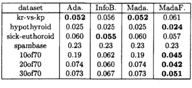
Table

1:

Test

errors

of boosting algorithms inthe

subsamplingframework.

Notethat l-of-k function andk/2-of-kfunction

cor-respond to $k$-disjunction and $k$-majority,

respec-tively. In [11], it isshown that InfoBoost

can

learn

r-of-k functions in$O(rk)$ steps whereas $\mathrm{A}\mathrm{d}\mathrm{a}\mathrm{B}\mathrm{o}\mathrm{o}\mathrm{s}\mathrm{t}$

needs $O(k^{2})$ stepswhen boolean literals

are

used

as

weak hypotheses. For $r=1,3,5$and$k=10$,

we

fix

a r-of-k function

over 100

boolean variables

as

the

target function,and

we

generate10,

000

random

ex-amples labeled by each r-of-k function, where the

random examples

are

drawn so that positive and

negative examples are equally likely. The size of

data

we use

varies$\mathrm{h}\mathrm{o}\mathrm{m}$about 3,000to 10,000.

For eachdataset, we prepare decisionstumps and the constant hypothesis +1 (i.e. the hypothesis

that always

answers

+1)

as

weak hypotheses. In

eachdataset, each record have nruneric attributes

orbinaryattributes. Foreachnumericattribute,

we

construct

a

decisionstump with

a

threshold,which

$\mathrm{p}\mathrm{r}\text{\’{e}} \mathrm{i}\mathrm{c}\mathrm{t}\mathrm{s}+1$ or-l depending

on

whether thevalue

of the attribute is

below

the

threshold

or

not. The threshold is chosen

so

that thetraining

error

of the

decision stump is minimized. For

each

binary

at-tribute,

we

prepare the decision stump which

an-swers

thevalue of theattribute.

We evaluate theboostingalgorithms by

cross

val-idation. We split each data randomly

10

times,

whereeach example is put into a training set with

probability

0.7

and

a

test set with with probability

0.3.

Foreachtraining set,

we

run

theboosting

algo-rithms in100stepsand evaluatetheir final

hypothe-ses on

the

test

data. The results

are

summarized in

As shown in Table5, performance of MadaFlat-appearsto becomparabletothoseof others

on

real

datasets. Also, MadaFlat is significantlybetter on

artificial datasets, as well

as

InfoBoost.

In the secondpart,

we

compare MadaBoost and

MadaFlatin the filteringframework. Basic settings

of our experiments in the filtering framework are

the

same as

those in the subsampling framework,

except the following: First ofall, in order to

ob-tainlarge datasets,

as

is done in [4],

we inflate

the

datasets by preparing

100

copies of each record in

the dataand changing their orderrandomly.

Con-sequently, the size of the inflated data varies ffom

300, 000 to 1, 000,000. Second, instead of running

each algorithm in

100

steps,

we

run

them until

theysample 10,0000examples. Moreprecisely, we

run

MadaFlatwith HSelect$(\epsilon, \delta)$, where parameter

$\epsilon=0.5$ and $\delta=0.1$

are

fixed. Also, we

run

Mad-$\mathrm{a}\mathrm{B}\mathrm{o}\mathrm{o}\mathrm{s}\mathrm{t}$with

geometric$\mathrm{A}\mathrm{d}\mathrm{a}\mathrm{S}\mathrm{e}\mathrm{l}\mathrm{e}\mathrm{c}\mathrm{t}$whoseparameters

are

$s=2,$ $\epsilon=0.5$and $\delta=0.1$

.

Third, note that

we use

heuristics for Lemma 1.

Although

Lemma

1 gives

a

theoretical guarantee

to approximatethepseudo gainaccurately enough,

it is too rough to

use

in practice. By using the central limittheorem, it isnot hard to show that A

isasymptoticallydistributed from$N(\Delta, \sigma^{2})$, where

$\sigma\leq 5\Delta/m$

.

This analysis implies that it is safe to

replacethe condition

on

$m$ inHSelect with

$m= \lceil\frac{10(\ln\pi_{\delta’}^{1}--\frac{1}{2}\ln\ln_{\sqrt{8\delta’}^{1)}}}{\Delta_{g}}\rceil$

.

Inthefollowing experiments,

we

usethis improved

heuristics.

Finally, in addition,

we

apply MadaBoost and

MadaFlatfor

text categorization tasks

on

a

collec-tion ofReuters news (Reuters-215782). We use the modified Apte$(” \mathrm{M}\mathrm{o}\mathrm{d}\mathrm{A}\mathrm{p}\mathrm{t}\mathrm{e}")$ split which

con-tains about 10,000

news

documents labeled with

topics. Wechoose twomajor topics(“$\mathrm{e}\mathrm{a}\mathrm{m}\mathrm{i}\mathrm{n}\mathrm{g}\mathrm{s}$” and

“acquisitions”) and for each of two topics, we let

boosting algorithms classify whether

a news

doc-ument belongs to the topic

or

not. As weak

hy-potheses,we prepare about 30,000decision stumps

correspondingto words. This experiment is donein

the

same

settingofprevious ones, exceptthatwedo

2_http:$//\mathrm{w}\mathrm{w}\mathrm{w}$.daviddlewis.$\mathrm{c}\mathrm{o}\mathrm{m}/\mathrm{r}\mathrm{o}\mathrm{e}\mathrm{o}\mathrm{u}\mathrm{r}\mathrm{c}\mathrm{e}\mathrm{s}/\mathrm{t}\mathrm{e}\epsilon \mathrm{t}\mathrm{c}\mathrm{o}\mathrm{l}\mathrm{l}\mathrm{e}\mathrm{c}\mathrm{t}\mathrm{i}\mathrm{o}\mathrm{n}\mathrm{s}$ $/\mathrm{r}\mathrm{e}\mathrm{u}\mathrm{t}\mathrm{e}\mathrm{r}\mathrm{s}21578$.

Table 2:

Test

errors

of boosting algorithms in the filtering

framework.

notinflatethisdataset. Theresults

are

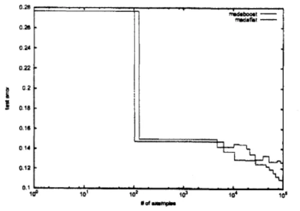
summarized inTable 5.

As

indicated in Table 5 and Figure 3, MadaFlatoften outperforms MadaBoost.

6 Summary and Rture Work

In this paper, we propose a modification of

$\mathrm{A}\mathrm{d}\mathrm{a}\mathrm{F}\mathrm{l}\mathrm{a}\mathrm{t}$ that

uses an information-theoretic

crite-rion for choosing hypotheses.

Our

preliminary

ex-periments show that

our

modification appears to

outperform MadaBoost in the filtering

framework.

As future work, advantages and noise torelance of MadaFlat

are

yet to be investigated theoretically.

Also,

we

plan to conduct experiments

over

much

larger data.

Acknowledgments

Thiswork is supported inpart by the $2\mathrm{l}\mathrm{s}\mathrm{t}$

cen-tury

COE

program at Graduate School of

Informa-tion Science and Electrical Engineeringin Kyushu University.

References

[1] J. A. Aslam. Improvingalgorithnts for

boost-ing. InProc. 13thAnnu.

_Confere

nce

on

Com-put. Leaming Theory,pages 200-207,

2000.

[2] Jose L. Balcazar, Yang Dai, and

Osamu

Watanabe. Provably fast training algorithms

boosting and applicationto agnosticlearning.

Joumal

_of

Machine Learning Research,

2003.

Figure

3:

Test error of boosinting algorithms for

Reuters-21578

data. The test

errors are

averaged

over

topics. The lower line correspondstothe test

error

ofh4adaF1at.

IEEE International

_Conference

on Data ${\rm Min}-$

ing (ICDM’Ol), pages43-50, 2001.

[3] C.L. Blake D.J. Newman, S. Hettich and C.J. Merz. UCI repository of machine learning

databases, 1998.

[4] C. Domingo, R.

Gavald\‘a,

and

O.

Watanabe. Adaptive sampling methods for scaling up

knowledge discovery algorithms. Data Mining

and Knowledge Discovery,$6(2):131-152$,

2002.

[5] C. Domingo and O. Watanabe. MadaBoost:

A modification of AdaBoost. In Proceedings

of

13th Annual

_Conference

on

Computational

Learning Theory, pages180-189,

2000.

[6] P. Domingos and G. Hulten. Mining

high-speeddata streams. In Prvceedings

_of

the Sixth

ACM Intemational

_Conference

on Knowledge

Discovery and Data Mining, pages 71-80, 2000.

[7] Y. Freund. Boosting

a

weaklearning algorithm

by majority.

_Information

and Computation,

$121(2):256-285$,

1995.

[8] Y. Freund and R. E. Schapire:. A

decision-theoreticgeneralization

of

on-line learningand

an

application to boosting. Joumal

_of

Com-puter and System Sciences, $55(1):119-139$,

1997.

[10] K. Hatanoand M. K. Warmuth. Boosting

ver-sus

covering. In Advances in Neural

Informa-tion Processing Systems 16, 2003.

[11] K. Hatano and O. Watanabe. Learning r-of-k

functions by boosting. In Prvceedings

_of

the 15th Intemational

_Conference

on

Algorithmic

Leaming Theory,

pages

114-126,

2004.

[12] M. Kearns and Y. Mansour.

On

the

boost-ing ability oftop-down decision tree learning

algorithms. Joumal

_of

Computerand System

Sciences, 58(1): 109-128, 1999.

[13] Michael J. Kearns, Robert E. Schapire, and

Linda Sellie. Towa.rd efficient agnostic

learn-ing. In COLT, pages 341-352,

1992.

[14] Yishay Mansour and David A. McAUaeter.

Boosting using branching programs. Joumal

of

Computerand System Sciences, $64(1):103-$

112,

2002.

[15] R. Meir and G. Rdtsch. An introduction to

boosting andleveraging. In Advanced lectures

on

machine leaming,

pages 118-183.

Springer-VerlagNew York, Inc,

2003.

[16] Robert E. Schapire. The strength of weak

learnability. Machine Leaming, $5(2):197-227$,

1990.

[17] Robert E. Schapire and Yoram Singer.

Im-proved boosting algorithms using

confidence-rated predictions. Machine Leaming,

$37(3):297-336$,

1999.

[18] R. A. Servedio. Smoothboostingandlearning

withmalicious noise. In

_14th

Annual

Confer-enceon Computational Leaming Theory, pages

473-489,

2001.

[19] L. G. Valiant. A theoryof the learnable.

Com-munications

_of

the ACM, $27(11):1134-1142$

,

1984.