Verified eigenvalue evaluation for Laplace operator on arbitrary polygonal domain (Mathematical foundation and development of algorithms for scientific computing)

(1)

Verified

eigenvalue

evaluation

for Laplace

operator

on

arbitrary

polygonal

domain

早稲田大学理工学術院/CREST,JST 劉雪峰 (Xuefeng Liu) 大石進一 (Shin’ichi Oishi)

Faculty ofScience and Engineering, Waseda University

Abstract

For eigenvalue problem of Laplace operator over polygonal domain $\Omega(\subset R^{2})$

of arbitrary shape, we proposed an algorithm based on finite element method

to bound the leading eigenvalues with indices guaranteed. The algorithm is

developed by welluseof max-min and min-max principles and newly constructed

a priori error estimation for FEM solution. The efficiency of the algorithm is

demonstratedby several computation examples.

1 Introduction

The eigenvalue problem of Laplacian has been well investigated in history from

various viewpoints. Here, we pay attention to giving accurate bounds for eigenvalues

with indices guaranteed. For such a purpose, Lehmann-Goerisch method is wellknown

as

a

effective way to give sharp bounds for eigenvalues

once a

quantity $\nu$ satisfying

$\lambda_{k}<\nu\leq\lambda_{k+1}$ is available, where $\lambda_{k}$ denotes the eigenvalues with increasing order

on

magnitude. To find such a $\nu$is not an easy work. In [8], M. Plum developed homotopy

method basedon operator comparison theorem to give acomputable lノ．As base problem

with explicit eigenvalues is necessary when we apply the homotopy method, domain

mapping is used to construct the base problem, which brings difficulties to solving

problems over general domain.

Inthis paper, startingfrom

an

earlyworkof Birkhoff, deBoor, Swartz andWendroff

[2], we propose a

new

method to give guaranteed estimation for leadingk-th eigenvalue

on arbitrary polygonal domain, where the finiteelement method(FEM) is used to give

approximate eigenvalues with computable error bounds. The estimate of $\lambda_{k}$ obtained

by using sparse domain triangulation will be relatively rough, but it can work

as

a

good candidate of ノ mentioned above $Thus$, if$needed$, the bounds can be sharpened

by further applying Lehmann-Goerisch method. The method proposed here can deal

with three types homogeneous boundary conditions associated with function space:

Dirichlet, Neumann and mixed

one.

To explain the method in a concise way, we only

showdetails for theDirichlet case. Also, it is possible toextend themethod for general

elliptic problem.

At the end of this paper, we show computation results on triangle and L-shaped

domain.

2 Preliminaries

$Let_{\mathfrak{l}}\zeta]$ be polygonal domain with arbitrary shape,

convex

or

non-convex.

We

in-troduce function space $V=H_{0}^{1}(\Omega)=\{v\in H^{1}(\Omega)|v=0 on \partial\Omega\}$. The notation $\Vert v\Vert_{L_{2}}$

(2)

$\mathcal{T}^{h}$ be

one

triangularization of $\Omega$, which

has

polygon boundary. The variational form

of eigenvalue problem is defined

as

below:

Find $\lambda\in R$ and $u\in V$ s.t. $(\nabla u.\nabla v)=\lambda(u, v)$, $\forall v\in V$. (1)

The classical continuous piecewise linear finite element(FE) space $V_{h}\subset V$ will be

used

as

approximation space. The Ritz method is to solve the variational problem in

$V_{h}$,

Find $\lambda^{h}\in R$ and _{$u_{h}\in V_{h}$} s.t. $(\nabla u_{h}, \nabla v_{h})=\lambda^{h}(u_{h}, v_{h})$ . $\forall v_{h}\in V_{h}$ . (2)

Supposing the bases of $V_{h}$ to be $\{\phi_{i}\}_{i=1}^{n}$, the problem of (2) is in fact a generalized

matrix eigenvalue problem:

$A^{h}x=\lambda^{h}B^{h}$, where $A_{i,j}^{h}=(\nabla\phi_{i}, \nabla\phi_{j})_{L_{2}},$$B_{i,j}^{h}=(\phi_{i}, \phi_{j})_{L_{2}}$ . (3)

The eigenvalues $\lambda_{k}^{h}$

can

be evaluated accurately by applyingverifiedcomputations, c.f.,

[1, 7, 9]. Denote by $\{\lambda_{i}, u_{i}\}$ (resp. $\{\lambda_{i}^{h},$$u_{i}^{h}\}$ ) the eigenpairs of (1) (resp. (2)) with

eigenfunction being orthogonallynormalized under $L_{2}$-norln. These eigenpairs

are

just

the stationary values and critical points of Rayleigh quotient on space $V$ (resp. $V_{h}$):

$R(u)$ $:=(\nabla u, \nabla u)/(u.u)$ . (4)

Since

an

upperbound for $\lambda_{i}$

as

$\lambda_{i}\leq\lambda_{i}^{h}$ is easytoobtain from min-maxprinciple, we

will pay attention to find satisfactory lower boundsfor eigenvalues. The eigenfunction

estimation will not be discussed here.

Let’s introduce two constants $C_{i,h}(i=0,1)$ to be used later, which are related to

function interpolations $\pi_{i}(i=0,1)$ over triangle element $K$. For $u\in L_{2}(K),$ $\pi_{0}u$ is

constant function s.t.

$\pi_{0}u\equiv\int_{K}u(x)dx/\int_{K}1dx$ , (5)

and for $u\in H^{2}(K),$ $\pi_{1}u$ is linear function s.t.

$(\pi_{1}u)(x)=u(x)$ on each vertex of K. (6)

Global interpolations$\pi_{0,h}$ and $\pi_{1,h}$

are

just the extension of $\pi_{0}$ and $\pi_{1}$. Define $h$ by the

mesh size and $C_{0,h}$ and $C_{1,h}$ the constants

over

triangulation $\mathcal{T}_{h}$,

$C_{i,h}$ $:= \max C_{i}(K)/h$ $(i=0,1)$ , (7)

$K\in \mathcal{T}^{h}$

where

$C_{0}(K):= \sup_{v\in H^{1}(K)\backslash \{0\}}|\pi_{0}u-u|_{L_{2}}/|u|_{H^{1}}$. $C_{1}(K):= \sup_{v\in H^{2}(K)\backslash \{0\}}|\pi_{1}u-u|_{H^{1}}/|u|_{H^{2}}$ .

3 Lower bound of eigenvalues

by

adopting

min-max

and

max-min

principle

In this section, we will introduce two methods to give lower bound for eigenvalues, all

of them adopting computable a priori estimate of Ritz-Galerkin solution of Poisson‘s

problem. Let $u\in H_{0}^{1}(\Omega)$ be the solution of following variation problem,

(3)

The solution $u\in H_{0}^{1}(\Omega)$, in meaning of distribution,

satisfies

the partial

differential

$equation-\triangle u=f$_. Whether$u$ belongs to $H^{2}(\Omega)$

or

notdepends

on

the domain shape.

Let $P_{h}$ be the orthogonal projection of _{$u\in V$} into

$V_{h}$,

$(\nabla u-\nabla P_{h}u, \nabla v_{h})=0$ $\forall v_{h}\in V_{h}$ . (9)

We will deduce a computable a apriori error estimate in the form as below,

$|u-P_{h}u|_{H^{1}}\leq M\Vert f\Vert_{L_{2}},$ _{$\Vert u-P_{h}u\Vert_{L_{2}}\leq M|u-P_{h}u|_{H^{1}}\leq\Lambda I^{2}\Vert f\Vert_{L_{2}}$} _, ₍₁₀₎

where $M$ is quantity to be evaluated _in Section _{4. In the} _{following, we} _{will introduce}

two methods to bound eigenvalues based onthis apriori error estimation.

3.1 Birkhoff

$s$

method:

application of

Min-Max

principle

Birkhoff, de Boor,

Swartz

and Wendroff [2] considered eigenvalue problem in form of

Rayleigh quotient $R(u)$ $:=N(u)/D(u)$ , where $N(u)$ and $D(u)$ are _quadratic forms of

$u\in V$ and _$D(u)>0$ for $u\neq 0$. Suppose $\{\lambda_{k}, u_{k}\}$ (resp. $\{\lambda_{h}^{k},$$u_{k}^{h}\}$) the stationary

values and critical points of $R(u)$ on space $V$ (resp. $V_{h}$), with increasing order on $\lambda_{k}$

(resp. $\lambda_{h}^{k}$). Birkhoff et al

deduced an

estimate for

$\lambda_{k}^{h}$ by applying Min-Max principle:

Theorem 1. Given any $v_{1}^{h},$$v_{2}^{h},$

$\cdots,$$v_{k}^{h}\in V_{h}(\subset V)$ satisfying $\sum_{i=1}^{k}D(v_{i}^{h}-u_{i})<1$, we

have,

_for

$k\geq 1$_,

$\lambda_{k}\leq\lambda_{h}^{k}\leq\lambda_{k}+(\sum_{i=1}^{k}N(v_{i}^{h}-u_{i}))/(1-(\sum_{i=1}^{k}D(v_{i}^{h}-u_{i}))^{1/2})^{2}$ (11)

For model problem of Laplacian in (1), $N(u)=(\nabla u, \nabla u)$ and $D(u)=(u, u)$. It

is natural to select $v_{i}^{h}=P_{h}u_{i}(i=1, \cdots, k)$ for each eigenfunction $u_{i}$, and apply the

error

estimate of (10):

$|u_{i}-P_{h}u_{i}|_{H^{1}}\leq M\Vert\triangle u_{i}\Vert_{L_{2}}=M\lambda_{i}\Vert u_{i}\Vert_{L_{2}}=M\lambda_{i}$ .

1

$u_{i}-P_{h}u_{i}\Vert_{L_{2}}\leq M|u_{i}-P_{h}u_{i}|_{H^{1}}\leq M^{2}\lambda_{i}$.

Thus, we obtain an a priori estimate for $\lambda_{k}^{h}$.

Theorem 2. Let $\lambda_{k}$ and$\lambda_{k}^{h}$ be the

ones

defined

inSeetion 2.

If

$1-l \downarrow I^{2}(\sum_{i=1}^{k}\lambda_{i}^{2})^{1/2}>0$,

we have

$\lambda_{k}^{h}\leq\lambda_{k}+M^{2}\sum_{i=1}^{k}\lambda_{i}^{2}/(1-M^{2}(\sum_{i=1}^{k}\lambda_{i}^{2})^{1/2})^{2}$ (12)

Define function $\phi_{1}$ on variable $t_{k}$ with parameters $\{t_{1}, \cdots, t_{k-1}\}$

as

below,

$\phi_{1}(t_{k};t_{1}, \cdots, t_{k-1}):=t_{k}+M^{2}\sum_{i=1}^{k}t_{i}^{2}/(1-\lrcorner\iota I^{2}(\sum_{i=1}^{k}t_{i}^{2})^{1/2})^{2}$ (13)

Noticing that $\phi_{1}$ is increasing

as

varible $t_{k}$ increases, $\phi_{1}(t_{k})$ has increasing inverse

function. Therefore, $\phi_{1}^{-1}(\lambda_{k}^{h};\lambda_{1}, \cdots , \lambda_{k-1})\leq\lambda_{k}$ . As $\lambda_{i}\leq\lambda_{i}^{h}$ for $i\geq 1$, we can further

see

(4)

Remark

3.1. In practical computation, instead

of

verifying $1- \lrcorner lI^{2}(\sum_{i=1}^{k}\lambda_{i}^{2})^{1/2}>0$,

we

will check astronger

condition

$1- \lrcorner\iota I^{2}(\sum_{i=1}^{k}\lambda_{i}^{h^{2}})^{1/2}>0$ since $\lambda_{i}^{h}(\geq\lambda_{i})s$

are

computable

ones.

Remark 3.2. Birkhoff, de Boor, Swartz and

_Wendroff

$[2J$ obtained the estimation

of

form

(11) with $V_{h}$ the space constructed by spline

functions.

By applying the error

estimate

_for

spline interpolation, quantitative estimate

_for

eigenvalue problem

_of

lD

Sturm-Liouville system is successfully done. However, it $\iota s$

difficult

to apply their

method to solve problem on general $2D$ domain. As a companson, our estimation in

Theorem 2 and 3can deal with eigenvalue problem with domain

_of

general shape, which

inhents advantages

_from

the

_finite

element method.

3.2 Bounding

eigenvalues

by

adopting

Max-Min

principle

Theorem3 (Liu). Let$v_{1}^{h},$$\cdots,v_{k-1}^{h}$ be arbitrary

functions of

$V_{h}$ and$V_{k-1}$ $:=span\{v_{1}^{h}, \cdots, v_{k-1}^{h}\}$.

Define

$\tilde{\lambda}_{k}$

by Rayleigh quotient on $V_{h}\cap V_{k-1}^{\perp}$ ($V_{k-1}^{\perp}$ : complement space

of

$V_{k-1}$ in $V$)

$\tilde{\lambda}_{k}=\min_{v_{h}\in V_{h}\cap V_{k-1}^{\perp}}\frac{(\nabla v_{h},\nabla v_{h})}{(v_{h},v_{h})}$.

Then, an a posteriori estimate

_for

$\tilde{\lambda}_{k}\iota s$ available,

$\tilde{\lambda}_{k}-\lambda_{k}\leq(l\mathfrak{l}I\tilde{\lambda}_{k})^{2}/(1+M^{2}\tilde{\lambda}_{k})$ (14)

where $M$ is the one in (10).

Proof.

From

Max-Min

principle,

we

have

$\lambda_{k}=\max W\subset V,\dim(W)\leq k-1$

$\min_{v\in W^{\perp}}\frac{(\nabla v,\nabla v)}{(v,v)}$ .

Thus, for specified $V_{k-1}$ $:=$ span$\{v_{1}^{h}, \cdots, v_{k-1}^{h}\}$, alower bound for $\lambda_{k}$ is given as

$\lambda_{k}\geq\min_{v\in V_{k-1}^{\perp}}\frac{(\nabla v,\nabla v)}{(v,v)}$. (15)

For any $v\in V_{k-1}^{\perp},$ $P_{h}v\in V_{h}$. Let $w_{h}$ be arbitrary

one

in $V_{k-1}(\subset V_{h})$. Then

$(\nabla v, \nabla w_{h})=0$. Thus $(\nabla P_{h}v, \nabla w_{h})=(\nabla v, \nabla w_{h})=0$, which implies that $P_{h}v\in$

$V_{h}\cap V_{k-1}^{\perp}$. Considering (10) and the definition of

$\tilde{\lambda}_{k}$

,

$\Vert v\Vert_{L_{2}}\leq\Vert P_{h}v\Vert_{L_{2}}+\Vert v-P_{h}v\Vert_{L_{2}}\leq\tilde{\lambda}_{k}^{-1/2}\Vert\nabla P_{h}v\Vert_{L_{2}}+\Lambda I\Vert\nabla(v-P_{h}v)\Vert_{L_{2}}$ .

$\Vert v\Vert_{L_{2}}^{2}\leq(\overline{\lambda}_{k}^{-1}+1\downarrow I^{2})(\Vert\nabla P_{h}v\Vert_{L_{2}}^{2}+\Vert\nabla(v-P_{h}v)\Vert_{L_{2}}^{2})=(\tilde{\lambda}_{k}^{-1}+1\mathfrak{l}I^{2})\Vert\nabla v\Vert_{L_{2}}^{2}$ .

Hence,

$\Vert\nabla v\Vert_{L_{2}}^{2}/\Vert v\Vert_{L_{2}}^{2}\geq\tilde{\lambda}_{k}/(1+\lrcorner \mathfrak{h}I^{2}\tilde{\lambda}_{k})$ for any $v\in V_{k-1}^{\perp}$ .

The equation (15) tells us,

$\lambda_{k}\geq\tilde{\lambda}_{k}/(1+1|I^{2}\tilde{\lambda}_{k})$ (16)

(5)

Remark 3.3. The subspace $V_{k-1}$ in Theorem 3

can

be taken as the

one

spanned by

first

$k-1$ eigenfunction

_of

(2). In this case, $\tilde{\lambda}_{k}=\lambda_{k}^{h}$ and lower bound

of

$\lambda_{k}$ is given

$as$;

$\lambda_{k}^{h}/(1+l|I^{2}\lambda_{k}^{h})\leq\lambda_{k}\leq\lambda_{k}^{h}$ . (17)

It is obvious that the above estimate based on Max-Minprinciple gives better estimate

than the one

_of

(11).

4 A

prioiri

_error

estimate

for Ritz-Galerkin

solu-tion

of

Poisson’s

problem

The following section will be devoted to evaluating $M$ appearing in a priori error

estimate (10) for projection $P_{h}$. The discussion will be divided into two parts, the

one with regular solution on convex domain and the one with singular solution on

non-convex

domain.

4.1 Convex

domain

First, we quote a well known result on a priori estimation for Laplacian.

Lemma 4. [4]Assume $\Omega$ is bounded convexpolygonal domain in $R^{2}$. For$u\in H^{2}(\Omega)\cap$

$H_{0}^{1}(\Omega)$ or$u\in H^{2}(\Omega)$ and$\partial u/\partial n=0$ on $\partial\Omega$, let _{$f$ $:=-\triangle u$}. Then, we have

$|u|_{H^{2}}\leq\Vert\triangle u\Vert_{L_{2}}=\Vert f\Vert_{L_{2}}$ .

Theorem 5. Let$\Omega$ be convexpolygonal domain and

$u$ be the solution

of

(8). The error

estimate

_for

$(u-P_{h}u)$ is given as

$|u-P_{h}u|_{H^{1}}\leq C_{1,h}h\Vert f\Vert_{L_{2}}$, $\Vert u-P_{h}u\Vert_{L_{2}}\leq C_{1,h}h|u-P_{h}u|_{H^{1}}\leq C_{1,h}^{2}h^{2}\Vert f\Vert_{L_{2}}$ .

Thus, we can take $M:=C_{1,h}h$ under current assumptions.

Proof.

Under the given assumptions, the solution $u$ belongs to $H^{2}(\Omega)$. By using

inter-polation error estimate for $\pi_{1,h}$ and the Lemma 4, wehave,

$|u-P_{h}u|_{H^{1}}\leq|u-\pi_{1,h}u|_{H^{1}}\leq C_{1,h}h|u|_{H^{2}}\leq C_{1,h}h\Vert f\Vert_{L_{2}}$ , (18)

where the constant $C_{1,h}$ is the

one

defined

in (7).

The

$L_{2}$

-norm error

estimation

can

be easily done by adopting Aubin-Nitsue’s technique.

$\square$

4.2 Non-convex domain

To deal with problem on

non-convex

domain, which has singular solution not

belong-ing to $H^{2}(\Omega)$, we adopt the hypercircle equation to deduce

a

computable

a

priori

error

estimate. Let $W^{h}$ be the lowest order Raviart-Thomas FEM space over domain

trian-gulation $\mathcal{T}^{h}$ and $\lrcorner lI^{h}$ the space ofpiecewise constant. Also, define subspace of _{$W_{h}$} for

$f_{h}$ in $M^{h},$ $W_{f_{h}}^{h}$ $:=\{p_{h}\in W^{h}|divp_{h}=f_{h}\}$. Recall the definition of

$\pi_{0,h}$ : $L_{2}(\Omega)arrow\Lambda I^{h}$

in Section 2,

(6)

From

the

definition,

we

have $\Vert u\Vert_{L^{2}}^{2}=\Vert\pi_{0,h}u\Vert_{L^{2}}^{2}+\Vert u-\pi_{0,h}u\Vert_{L^{2}}^{2}$and

$\Vert u-\pi_{0,h}u\Vert_{L^{2}}\leq C_{0,h}h|u|_{H^{1}}$ if $u\in H^{1}$.

where $C_{0,h}$ is the constant defined in (7).

Let’s introduce acomputable quantity $\kappa$

over

finite dimensional spaces:

$\kappa:=\max_{hf\in\Lambda I^{h}\backslash \{0\}}$ $\min_{v_{h}\in V_{h}}\min_{p_{h}\in W_{f_{h}}^{h}}\Vert p_{h}-\nabla v_{h}\Vert_{L_{2}}/\Vert f_{h}\Vert_{L_{2}}$ (19)

Lemma 6. Given $f_{h}\in M^{h}$, let $\tilde{u}\in H^{1}$ and _{$\tilde{u}_{h}\in V_{h}(\subset V)$} be the solutions

of

_{$var\iota a-$}

tionalproblems,

$(\nabla\tilde{u}, \nabla v)=(f_{h}, v)$, $\forall v\in V$ . $(\nabla\tilde{u}_{h}, \nabla v_{h})=(f_{h}, v_{h})$, $\forall v_{h}\in V_{h}$ , (20)

respectively. Then we have a computable error estimate as below:

$|\tilde{u}-\tilde{u}_{h}|_{H^{1}}\leq\kappa\Vert f_{h}\Vert_{L_{2}}$ . (21)

Proof.

From Prager-Synge’stheorem, wehave, for$\tilde{u}$in (20) and any _{$v_{h}\in V_{h},$}_{$p_{h}\in W_{f_{h}}^{h}$},

such a hypercircle equation holds,

$\Vert\nabla\tilde{u}-\nabla v_{h}\Vert_{L_{2}}^{2}+\Vert\nabla\tilde{u}-p_{h}\Vert_{L_{2}}^{2}=\Vert p_{h}-\nabla v_{h}\Vert_{L_{2}}^{2}$. (22)

Thus,

$\Vert\nabla\tilde{u}-\nabla v_{h}\Vert_{L_{2}}\leq\Vert\nabla v_{h}-p_{h}\Vert_{L_{2}}$, $\forall v_{h}\in V_{h},$ $\forall p_{h}\in W_{f_{h}}^{h}$ . (23)

From minimization principle and the definition of$\kappa$, we obtain

$\Vert\nabla\tilde{u}-\nabla\tilde{u}_{h}\Vert_{L_{2}}\leq\min_{v_{h}\in V_{h}}\min_{p_{h}\in W_{f_{h}}^{h}}\Vert p_{h}-\nabla v_{h}\Vert_{L_{2}}\leq\kappa\Vert f_{h}\Vert_{L_{2}}$ . (24)

$\square$

Theorem 7. For any $f\in L_{2}(\Omega)$, let $u\in V$ and $u_{h}\in V_{h}$ be solution

of

$var\cdot lational$

problems

$(\nabla u, \nabla v)=(f, v)$, $\forall v\in V$, $(\nabla u_{h}, \nabla v_{h})=(f, v_{h})$, $\forall v_{h}\in V_{h}$ . (25)

respectively. Introduce quantity $M:=\sqrt{C_{0h}^{2}h^{2}+\kappa^{2}}$, where $C_{0,h}$ is the constant

defined

in (7). Then, we have,

$|u-u_{h}|_{H^{1}}\leq M\Vert f\Vert_{L_{2}}$, $\Vert u-u_{h}\Vert_{L_{2}}\leq l\mathfrak{l}I^{2}\Vert f\Vert_{L_{2}}$ . (26)

Remark 4.1. The quantity $\Lambda I$, independent

of

$f$, will $dec\uparrow ease$ when mesh $is\uparrow efined$.

By theoretical analysis, we can show that $\Lambda I$ tends to $0$ in the

same

order

as

the

error

of

linear conforming $FEM$solution solution.

Proof.

We follow analogous framework with $I\backslash$’ikuchi and Saito [6] to finish the proof.

Let $\tilde{u}$ and $\tilde{u}_{h}$ be the

ones

defined in Theorem 6 with $f_{h}=\pi_{0,h}f$. The minimization

principle leads to $|u-u_{h}|_{H^{1}}\leq|u-\tilde{u}_{h}|_{H^{1}}$ . Decomposing $u-\tilde{u}_{h}$ by $(u-\tilde{u})+(\tilde{u}-\tilde{u}_{h})$,

we have

(7)

From

the

definitions

of$u$ and $\tilde{u}$,

we

have, for any $v\in V$

$(\nabla(u-\tilde{u}), \nabla v)=(f-\pi_{0,h}f, v)=((I-\pi_{0,h})f, (I-\pi_{0,h})v)$ .

Taking $v$ to be $u-\tilde{u}$ and applying the

error

estimate of interpolation

$(I-\pi_{0,h})v$,

$|u-\tilde{u}|_{H^{1}}\leq C_{0,h}h\Vert(I-\pi_{0,h})f\Vert_{L_{2}}$ . (28)

Substitute (21) and (28) into (27),

$|u-u_{h}|_{H^{1}}\leq C_{0,h}h\Vert(I-\pi_{0,h})f\Vert_{L_{2}}+\kappa\Vert\pi_{0,h}$

fli

$L_{2}\leq\sqrt{C_{0h}^{2}h^{2}+\kappa^{2}}\Vert f\Vert_{L_{2}}$ .

The estimate for $\Vert u-u_{h}\Vert_{L_{2}}$

can

be easily done by applying

Aubin-Nitsche’s

method.

$\square$

5 Computation

The computation of quantity $\kappa$ turns to solving eigenvalue problem of matrix, for

which weomit thedetails but point out that evaluationof$\kappa$

consumes

most ofthe total

computationtime. To obtain accurate numerical result, weadopt interval computation

arithmetic to do the floating-point computation. The total framework is

as

below

1$)$ Tlriangulate the domain $\Omega$ andconstruct finite element space

$V_{h}$.

2$)$ Solve eigenvalues problem $A^{h}x=\lambda^{h}B^{h}x$ under the bases of

$V_{h}$.

3$)$ Evaluate quantity $M$ for the mesh and domain.

4$)$ Calculate the lower and upper bounds of

$\lambda_{k}$ by using (12) or (17).

In the following we display computation examples on several domains.

5.1 Triangle domain

In

case

_{of unit isosoceles right triangle domain, due to the}symmetryofspecified triangle

domain,

we can

apply reflecting techniques, $e.g.,[5]$_{, to}obtain the explicit eigenpairs

as

below:

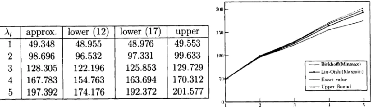
$\{\lambda=m^{2}+n^{2}, u=\sin m\pi x\sin 7?\pi y-\sin\uparrow?\pi x\sin m\pi y\}_{m>n\geq 1}$.

To compare the efficiency of the methods basing

on

Max-min principle and the

Min-max principle, we display the estimates of (12) and (17) in Table 1.

5.2 Computation

Results

on

L-shaped domain

Thedomain is taken

as

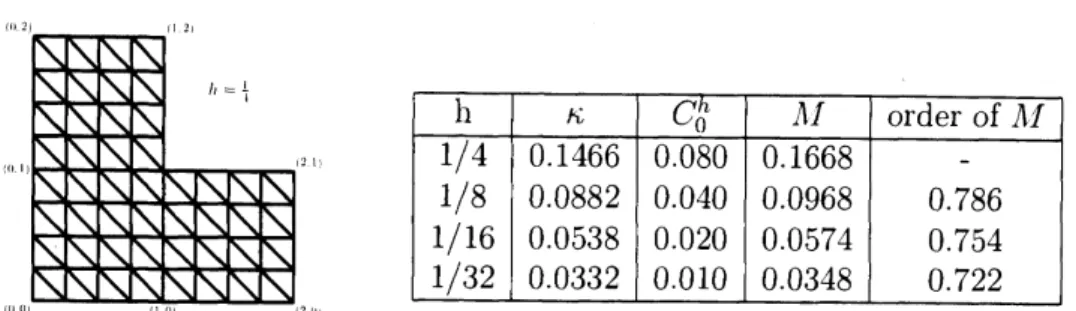
$\Omega=[0,2]\cross[0.2]\backslash [1,2]\cross[1,2]$. As amodel problem, it hasbeen

well explored by many people, e.g., L. Fox, P. Henrici and C. Moler [3]. However, to

the author$s$ knowledge, most of the results are given only in the senseof approximate

computation. _{Although our} _{method gives} _a _{relatively rough evaluation, it} _can _easily

deal with more general domain and the result works as mathematically correct with

(8)

Table 1: Estimates by Min-max(12) and Max-min (17) principle. $(h=1/32)$

Table 2: Eigenvalue estimates for Laplacian ontriangle domain (Dirichlet b.d.$c.$)

In Table 4,

we

list the first 5 eigenvalues given by [3] and the verified

bounds

by

our

proposed method. The values of $\kappa,$ $C_{0}^{h}$ and $M$, which

are

only depending

on

the

mesh, are displayed in Table 3. We can see $M$ tends to zero in order less than 1. Once

lower bound for $\lambda_{5}$ is available,wecanfurther apply the Lehmann-Goerischmethod to

obtain more precise bound for $\lambda_{1},$

$\cdots,$$\lambda_{4}$. Such

a

computation, although not verified,

has been reported by Yuan and He [10] with very sharp bounds, while thelower bound

for $\lambda_{5}$ is obtained in

a

different way.

6 Conclusion

For the classical eigenvalue problems of Laplace operator over 2-dimensional

do-main, we have proposed a novel and robust method to give accurate lower and upper

bounds for eigenvalues. The method can deal with both

convex

and

non-convex

do-mains with general shape. To apply the Lehmann-Goerischmethod for purposeof high

precision,

we

still need pay efforts

on

constructingbase functions

over

general domain.

Acknowledgement

The authors would like show great appreciation to Prof. M. Plum and Prof. K.

(9)

$|(|$ $|1(|$

Table 3: Uniform mesh of L-shaped domain and $\kappa$ values

Table 4: Eigenvalue evaluation for L-shaped domain $(h=1/32)$

References

[1] H. Behnke. The calculation of guaranteed bounds foreigenvaluesusingcomplementary variational

principles. Springer-Verlag, 47(1): 11-27, 1991.

[2] G. Birkhoff, C. De Boor, B. Swartz, and B. Wendroff. Rayleigh-ritz approximation by piecewise

cubic polynomials. SIAM JoumalonNumerical Analysis, pages 188-203, 1966.

[3] L.Fox, P.Henrici,andC.Moler. Approximations and bounds for eigenvalues ofelliptic operators.

SIAM Joumal on NumericalAnalysis, $4(1):89-102$, 1967.

[4] P. Grisvard. Elliptic problems in nonsmooth domains. Pitman, 1985.

[5] F. Kikuchi and X. Liu. Determination of the Babu\v{s}ka-Aziz constant for the linear triangular

finite element. JapanJoumal _ofIndustnal andApplied Mathematics, 23.75-82, 2006.

[6] F. Kikuchi and H. Saito. Remarks on aposteriori errorestimation for finite element solutions.

Journal _ofComputational and Applied Mathematics, 199.329-336,2007.

[7] K.Maruyama, T. Ogita,Y. Nakaya, andS. Oishi. Numericalinclusionmethod for all eigenvalues

of real symmetric definite generalized eigenvalue problem. IEICE Trans, J97-A(8):1111-1119,

2004.

[8] M. Plum. Bounds for eigenvalues ofsecond-order elliptic differential operators. The Joumal _of Applied Mathematics andPhysics(ZAMP), 42(6) 848-863, 1991.

[9] N. Yamamoto. A simple method for errorbounds ofeigenvalues of symmetric matrices. Linear Algebra and its Applications,$324(1-3).227-234$ , 2001.

[10] Q. Yuan and Z. He. Bounds to eigenvalues of the laplacian on L-shaped domain byvariational methods. Joumal_ofComputational and AppliedMathematics, $233(4):1083-1090$ , 2009.