ソリトン理論の最近の話題 : 超離散の応用と交通流 (力学系理論の展開と応用)

ソリトン理論の最近の話題一超離散の応用と交通流

-Recent development

in Soliton

theory

-

Ultradiscrete

method and

its

applications-龍谷大学理工学部 西成 活裕(Katsuhiro Nishinari)

Dept.

of Info.

Math., Ryukoku

University 1

One dimensional cellular automaton (CA) models of vehicle traffic and ant traffic

are

proposed in this paper. These models

are

closely related to the Burgers $\mathrm{C}\mathrm{A}$, which is

known

as an

integrableCAderived by using the ultradiscretemethod. Differencesbetween

vehicleand ant traffic

come

from mainly theexistenceof pheromone in the ant trailmodel,

which allows long

range

interactionfor ants. In the caseof vehicle traffic, it is important

toconsider socalled synchronizedstate, where both flow and density

are

high. The model

proposed in this

paper

is shown toreproduce this state around the critical density.

1

Introduction

Trafficproblems have beenattractingnotonly engineers but also physicists [1]. Especially

it has been widely accepted that the phase transition from free to congested traffic flow

can

be understood using methods from statistical physics $[2, 3]$

.

In recent years cellular

automata(CA) $[4, 5]$ have been used extensively to study traffic flow in this context. Due

to theirsimplicity, CA models have also been applied byengineers, e.g.for the simulation

ofcomplex traffic systemswith junctions and

traffic

signals [6]. Many traffic

CA

models

have been proposed so far [2, 7, 8], and

among

these $\mathrm{C}\mathrm{A}$

,

the deterministic rule 184 CA

model (R184),which is

one

of

theelementary

CA

classified by

Wolfram

[4],is the prototype

of all traffic CA models. R184 is known to represent the minimum movement of vehicles

in

one

lane and shows

a

simple phasetransition from freetocongestedstateoftraffic flow.

In

a

previous

paper

[9], using the ultra discrete method [10], the Burgers CA (BCA) has

been derived from the Burgers equation

$v_{t}=2vv_{x}+v_{xx}$

,

(1)

57

which was interpreted as a macroscopic traffic model [11]. The BCA is written using the

minimum function $\min$ by

$U_{j}^{t+1}=U_{j}^{t}$ $+$ $\min\{U_{j-1}^{t}, L-U_{j}^{t}\}-$ $\min\{U!, L-U_{j+1}^{t}\}$, (2)

where $U_{j}^{t}$ denotes the number of vehicles atthe site$j$ andtime $t$

.

If

we

put therestriction

$L=1,$ it

can

be easily shown that the

BCA

is equivalent toR184. Thus

we

haveclarified

the connection between theBurgers equation and R184,which offers better understanding

of the relation between macroscopic and microscopic models. The BCA given above is

considered as the Euler representation of traffic flow. As in hydrodynamics there is

an

another representation, called Lagrange representation [12], which is specifically used for

car-following models. The Lagrange version of the

BCA

is given by [13]

$x_{\dot{1}}^{t+1}=x_{1}^{t}$. 1 $\min\{V_{\max}, x_{\dot{\iota}+S}^{t}-x_{*}^{t}. -S\}$, (3)

where $V_{\max}=S=L$ and $x_{1}^{t}$. is the position of $i$-th car at time $t$

.

Note that in (3) $S$

corresponds a “perspective” or anticipation parameter [14] which represents the number

of

cars

that

a

driver

sees

in front, and $V_{\max}$ is themaximumvelocity ofcars. (3) is derived

from the

BCA

mathematically byusing

an

Euler-Lagrange

(EL)

transformation

[13] which

is a discrete version of the well-known EL transformation in hydrodynamics.

2

A

new

traffic

model

In thissection we will develop theBCA (3) to a

more

realistic model by introducing

slow-tostart $(\mathrm{s}2\mathrm{s})$ effects [15, 16, 17, 18] and a driver’s perspective $S$

.

First, let us extend (3)

tothe case $V_{\max}\mathrm{z}$$S$ andcombine it with the$\mathrm{s}2\mathrm{s}$model. The$\mathrm{s}2\mathrm{s}$model [12] iswritten in

Lagrange form

as

$x:+$’ $=$ $x_{i}^{t}+ \min\{1, x:_{+1}-x_{i}^{t}- 1, x_{i+1}^{t-1}-x_{\dot{l}}^{t-1}-1\}$

.

(4)

Note thatthe inertiaeffect ofcars is taken into account in this model. Now by combining

(3) and (4)

we propose a new

Lagrange model with general $S$

as

follows:

$x_{\dot{1}}^{t+1}$ _$=$ $x_{}^{t}+ \min\{V_{}^{t},\min_{k=1,\cdots,\mathrm{S}-1}(x_{i+k}^{t}-x_{\dot{\iota}}^{t}-k +V_{i+k}^{t})$$\}$, (5)

where the last term represents thecollision-free condition, and

The condition thatthere is

no

collision between the$i$-th and$i+k$-thcars $(k=1, \cdots, S-1)$

is given by

$x_{*+k}^{t}.-x\mathrm{i}$ $-k+V_{*+k}^{t}.\geq V_{}^{t}$, (7)

for $S\geq 2$ (if $5=1$ then

we

simply put $k=1$), which is identical tothelast term in (5).

In

contrast

to the

NS

model, the velocity ofthe preceeding

car

is taken into account in

the

calculation

of the safe velocity, i.e.

our

model

also

includes

anticipation

effects.

3

Metastable

branches

and their

stability

Next, we investigate the

fundamental

diagram of this

new

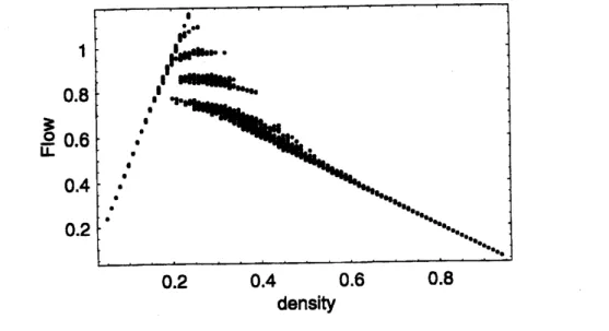
hybrid model. In Fig. 1,

we

Figure 1:

Fundamental

diagramofthe

new

Lagrange model. Parameters

are

set to$V_{\max}=$

$5$ and $S=2,$ and the spatial period is 100 sites. The initial

car

density is varied from

0.05 to

0.95

in steps of

0.01.

At each density,

we

start calculations from 30 randomly

generated initial

configurations, and show only the data at the time $t=100.$

We

observe

given

1 metastabl

$\mathrm{e}$ branches in the detqrministic

case.

The fluctuations of the branches

show the fact that theasymptotic flow of the systemsometimes becomes periodic

instead

of stationary between $0.2\leq\rho\leq 0.5.$

observeacomplex phase transition from

a

free tocongested state

near

the critical density

0.2\sim 0.4. There are many metastable branches in the diagram, similar to

our

previous

models i$\mathrm{n}$ Euler form $[19, 20]$

or

in other models with anticipation [21]. We also point

out that there is

a

wide scattering

area near

the critical density in the observed data[22]

which

may

be

related

to these

metastable

branches. These branches mayaccount for

some

aspects of the scattering

area

observed empirically.

59

branches we find phase separationinto a free-flow and a jamming region. In the former,

pairs

move

with velocity $v_{f}$ and aheadwayof$d_{f}$ emptycells between consecutive pairs. In

thejammed region, the velocityof thepairs is$v_{j}$ and the headway $d_{j}$

.

$N_{j}$ and $N_{f}$

are

the

numbersof

cars

in the jamming

cluster

and the free uniformflow, respectively. We

assume

$N_{f}$ and $N_{j}$ tobe even

so

that thereare$N_{f}/2$and $N_{j}/2$pairs, respectively. Then the total

number of

cars

$N$ is given by _{$N=N_{j}1N_{f}$} and the total length of the system becomes

$\mathit{1}=(d_{j}+2)N_{j}/2+(d_{f}+ 2)$Nj/2. Since the average velocity is $\overline{v}=\{NfVf+NjVj)/N$

and density and flow of the system are given by $\rho=N\oint l$ and $Q=\rho\overline{v}$, we obtain the

flow-density relation

as

$Q=2 \frac{vf-v_{j}}{d_{f}-d_{j}}+(v_{j}-(d_{j}+2)\frac{v_{f}--v_{j}}{d_{f}d_{j}})\rho$

.

(8)

It is shown that these branches are generally unstable to perturbations like braking[23].

4

The

ant-trail

model(ATM)

Theantscommunicatewith each other by droppingachemical (genericallycalledpheromone)

on the substrate as they crawl forward [24]. Although we cannot smell it, the trail

pheromone sticks to the substrate long enough for the other following sniffing ants to

pick up its smell and follow thetrail. Ant trails may

serve

different purposes (trunk trails,

migratory routes) and may also be used in

a

different way by different species. Therefore

oneway trails

are

observed

as

well

as

trails with counterflow of ants.

In [25] we developed a particle-hopping model, formulated in terms of stochastic$\mathrm{C}\mathrm{A}$,

which may be interpreted

as a

model ofunidirectional flow in an ant-trail. Asin ref. [25],

rather than addressing the question ofthe emergence of the ant-trail, we focus attention

here

on

the traffic ofants

on

a trail which has already been formed.

Herewe define the model which was originally introduced in ref.[25]. Each site of

our

one

imensional ant-trail model represents

a

cell that

can

accomodateat most

one

ant at

a time (seeFig. 2). The lattice sites are labelled by theindex $i(i=1,2, \ldots, L);L$ being the

lengthofthe lattice. We associate two binary variables $S_{\dot{l}}$ and $\sigma$

:

with each site$i$where $S_{1}$.

takes the value0

or

1depending

on

whether the cell is empty

or

occupied by

an

ant.

Simi-larly, $\sigma i=1$if the cell $i$contains pheromone; otherwise, $\mathrm{y}_{i}=0.$ Thus,

we

have two subsets

ofdynamicalvariablesinthismodel, namely, $\{S(t)\}\equiv\{\mathrm{S}(\mathrm{t})\}S_{2}(t)$,$\ldots$,$S_{i}(t)$,$\ldots$,$S_{L}(t))$ and $\{\mathrm{S}(\mathrm{t})\}\equiv(\sigma_{1}(t), \sigma_{2}(t)$,$\ldots$,$\sigma:(t)$,$\ldots$,$\sigma$z(t)$)$

.

The instantaneous state (i.e., the configuration)

of the system at any time is specified completely by theset $(\{5\}, \{\sigma\})$

.

which may be interpreted

as

amodel ofunidirectional flow in an ant-trail. Asin ref. [25],

rather than addressing the question ofthe emergence of the ant-trail, we focus attention

here

on

the traffic ofants

on

atrail which has already been formed.

Herewe define the model which was originally introduced in ref.[25]. Each site of

our

one-dimensional ant-trail model represents

a

cell that

can

accomodateat most

one

ant at

a time (seeFig. 2). The lattice sites are labelled by theindex $i(i=1,2, \ldots,L);L$ being the

lengthofthe lattice. We associate two binary variables $S_{\dot{l}}$ and $\sigma$

:

with each site$i$where $S_{1}$.

takes the value0

or

1depending

on

whether the cell is empty

or

occupied by

an

ant.

Simi-larly, $\sigma i=1$if the cell $i$contains pheromone; otherwise,$\sigma i=0$

.

Thus,

we

have two subsets

ofdynamicalvariablesinthismodel, namely, $\{S(t)\}\equiv(S_{1}(t),S_{2}(t),$ $\ldots$,$S_{i}(t)$,$\ldots,S_{L}(t))$and

$\{\sigma(t)\}\equiv(\sigma_{1}(t), \sigma_{2}(t)$,$\ldots$,$\sigma:(t)$,$\ldots$,$\sigma L(t))$

.

The instantaneous state (

$\mathrm{i}.\mathrm{e}.,$ the configuration)

$\cap \mathrm{q}$ $\cap \mathrm{Q}$ $\cap \mathrm{q}$ $\mathrm{S}(\mathrm{t}$} ants $\sigma(\mathrm{t})$ pheromone $\mathrm{a}\mathrm{n}\alpha$ pheromone ants phmrnone $*\mathrm{m}\mathrm{I}\mathrm{w}\mathrm{n}\mathrm{e}$ $\mathrm{a}\mathrm{n}\mathrm{t}s\mathrm{P}^{\mathrm{h}\mathrm{m}\mathrm{t}\mathrm{n}\mathrm{o}\mathrm{n}\mathrm{e}}$

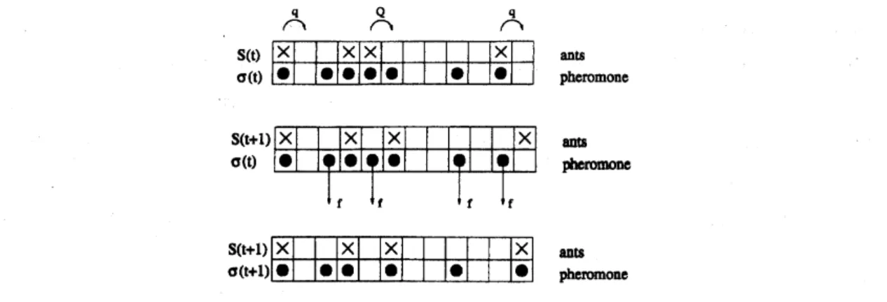
Figure 2: Schematic representation of typical configurations; it also illustrates the

up-date procedure. Top: Configuration at time $t$, i.e.

before

stage I of the update. The

non-vanishing hopping probabilities of the ants

are

also shown explicitly. Middle:

Config-uration

_after

one possible realisation ofstage $I$

.

Two ants have moved compared to the

top part of the figure. Also indicated arethe pheromonesthat may evaporatein stage $II$

of the update scheme. Bottom: Configuration

_after

one

possible realization of stage $II$

.

Twopheromones haveevaporated and

one

pheromonehas been created due to the motion

of

an

ant.

Since

a

unidirectional motion is assumed, ants do not

move

backward. Their

forward-hopping probability is higher if it smells pheromone ahead of it. The state of the system

is updated at each time step in two stages. In stage I ants

are

allowed to

move.

Here the

subset$\{S(t+1)\}$atthetime step$t+1$ isobtained using the full information$(\{S(t)\},$$\{\mathrm{v}(\mathrm{t})\}$

at time $t$

.

Stage II corresponds to the evaporation of pheromone. Here only the subset

$\{\mathrm{v}(\mathrm{t})\}$isupdated

so

thatatthe end of stageIIthe

new

configuration $(\{S(t+1)\}, \{\sigma(t+1)\})$ at time $t+1$ is obtained. In each stage the dynamical rules

are

applied in parallelto all

ants and pheromones, respectively.

Stage I.$\cdot$ Motion

of

ants

An ant in cell $i$ that has

an

empty cell in front ofit, i.e., Si(t) $=1$ and _{$S_{i+1}(t)=0,$} hops

forward with

probability $=\{$ $Q$ if $\sigma:+1(t)=1,$ (9)

$q$ $i$ $\sigma_{\dot{|}+1}(t)=0,$

where, to be consistent with real ant-trails, we

assume

$q<Q.$

Stage $\mathrm{I}\mathrm{I}$

.

Evapo ration

of

pheromones

At each cell $i$occupied by

an

ant after stage I

a

pheromone will be created, i.e.,

61

$\mathrm{g}$

$e_{2}\mathrm{o}\mathrm{e}5,\ovalbox{\tt\small REJECT}_{4}$

$\mathrm{D}\mathrm{e}\mathrm{n}\mathrm{a}[] \mathrm{y}$

(a)

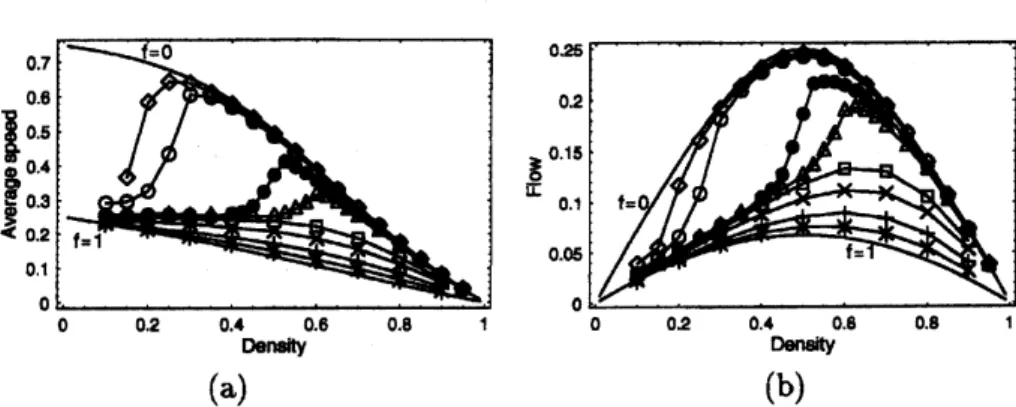
Figure 3: Theaverage speed (a),flux (b) of theants,extracted fromcomputersimulation

data,areplotted againsttheir densities fortheparameters$Q=0.75$,$q=$ 0.25. The discrete

data points correspondingto$f=$ 0.0005(0), 0.001(0),0.005(0), 0.01(A), 0.05(D), 0.10(x),

0.25(+),0.50(*) have beenobtained fromcomputersimulations; thelines connecting these

data points merelyserve as the guideto the eye. In (a) and (b), the

cases

$f=0$and $f=1$

are

also displayed, which correspond to the

NS

model with qeff $=Q$ and $\mathrm{g}$, respectively.

On the other hand, any ‘free’ pheromone at asite $i$ not occupied by

an

ant will evaporate

with the probability $f$ per unit time, i.e., if$S\{(t+1)=0$,(Ti(t) $=1,$ then

$\sigma_{i}(t+1)=\{$ 0 with probability

$f$,

(11)

1 with probability $1$

-f.

Note that the dynamics conserves the number $N$ of ants, but not the number of

pheromones.

The rules

can

be written in

a

compact form

as

thecoupled equations

Note that the dynamics conserves the number $N$ of ants, but not the number of

pheromones.

The rules

can

be written in

a

compact form

as

thecoupled equations

$S_{j}(t+1)$ $=$ $S_{j}(t)+ \min$($\eta_{j-1}(t)$,Sj $\{\mathrm{t}$), 1-Sj$( \mathrm{t})-\min$($\eta_{j}(t)$,Sj$\{\mathrm{t}$), $1-S_{j+1}(t)\phi 12)$

Sj$(\mathrm{t}+1)$ $=$ Sj$(\mathrm{t}+1),$$\min(\sigma_{j}(t),\xi_{j}(t)))$, (13)

where $\xi$ and 7

are

stochastic variables defined by $4_{\mathrm{i}}(t)$ $=0$ with the probability $f$ and

Sj(t) $=1$ with 1 –f, and Sj(t) $=1$ with _the probability $p=q+(Q-q)\sigma_{j+1}(t)$ and

(Ti(t) $=0$ with l-p. This representation is useful for the development ofapproximation

schemes.

The flux $F$ and the average speed $V$ of

vehicles

are

related by the hydrodynamic

relation $F=$ pV. The density-dependence of the

average

speed in

our

ATM is shown

in Fig. $3(\mathrm{a})$

.

Over a range

of small values of $f$, it exhibits an anomalous behaviour

in the

sense

that, unlike

common

vehicular traffic, $V$ is not

a

monotonically decreasing

function of the density $\rho$

.

Instead

a

relatively sharp

crossover

can be observed where the

speed increaseswith thedensity. A proper theory oftheATMshould reproduce the

non-monotonic variation of the average speed with density (shown in Fig. $3(\mathrm{a})$) and, hence,

5

Zero Range Process

It is known that the

zero

range

process(ZRP) is

one

of the exactly solvable stochastic

models. It is a process that the particle hopping probability is realted to the number of

gaps

in front. Thus it is closely related to

our

ATM, since the hopping probability $u$ ofan

ant is given by

$u(x)=q+(Q-q)g(x)$ (14)

where we take $g(x)=(1-f)^{x/v}$_, $x$ is the

gaps

and $v$ is the

mean

velocity of ants. Thus

by usingthe ZRP, the

average

velocity $v$ ofants is calculated by

$v= \sum_{x=1}^{L-M}u(x)p(x)$ (15)

where $L$ and $M$

are

the system size and the number of ants respectively (hence $M/L$ is

the density), and

$p(x)=h(x) \frac{Z(L-x-1,M-1)}{Z(L,M)}$

,

(16)

where $Z$is the partition function and $h(x)$

can

be calculated as[27]

$h(x)=\{$

1-u(l) for $x=0$

$\frac{1-u(1)}{1-u(x)}\prod_{y=1}^{x}\frac{1-u(y)}{u(y)}$ for $x>0$ (17)

The partition function $Z$ is obtained by the

recurrence

relation

$Z$($L$Jf) $= \sum_{x=0}^{L-M}Z$(

$L-x-$

1Jf

-l)h(a), (18)

with $Z(x, 1)=h(x$- 1$)$ and $Z$(x,$x$) $=$ h(x).

By using theseformulae,

we

obtain the following fundamental diagram. We could set

at most $L=200$ up to

now

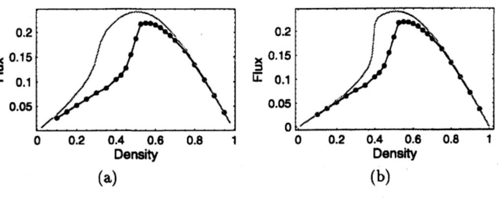
because ofthe numerical precision restriction. Fundamental

diagram of ATM is given by the figure 4. The blackcurvewith circlesis the numerical data,

and the simple black

curve

is the theretical

curve

calculated by using ZRP. Systemsize is

$L=100(\mathrm{F}\mathrm{i}\mathrm{g}.4(\mathrm{a}))$and $L=200(\mathrm{F}\mathrm{i}\mathrm{g}.4(\mathrm{b}))$

.

Parameters

are

$Q=0.75$,_$q=$0.75,$f=$

0.001.

We

see

that the theoretical

curve

approaches to the numerical

one

if

we

take lager $L$’s.

6

Concluding discussions

In thispaper we have proposed a new hybrid model of traffic flow of Lagrange type which

B3

$\cup’.d$ $l^{f}$ $n\mathrm{r}\epsilon$ 0.1 0.05 0 0.2 0.4 0.6 0.8 1 0 $\mathrm{n}\mathrm{s}$

.

(a) (b)

Figure 4: Comparison ofthe results by using ZRP with simulations in the

case

of $(\mathrm{a})Z=$

$100$ and $(\mathrm{b})Z=200.$

branches around the critical density in its fundamental diagram. The upper branches

are

unstable and will decrease its flow under perturbations. Moreover, we have shown a

new

ant traffic model by taking into account the effect of pherornone. The fundamental

diagramshowsunusual velocity-density relation, which is analyzed by using the

zero

range

process.

References

[1] D. Helbing and H.J. Herrmann and M. Schreckenberg and D. E. Wolf $(\mathrm{e}\mathrm{d}\mathrm{s}.)$,“Traffic

and Granular Flow ’99”, (Springer, 2000, Berlin).

[2] D. Chowdhury, L. Santen and A. Schadschneider, Phys. Rep. 329 (2000) 199.

[3] D. Helbing, Rev. Mod. Phys., 73 (2001) 1067.

[4] S. Wolfram, Theory and applications

_of

cellular automata, (World Scientific, 1986,

Singapore).

[5] B. Chopard and M. Droz, Cellular Automata Modeling

_of

Physical Systems,

(Cam-bridge University Press, 1998).

[6]

S.

Bandini, R. Serra and F.

S.

Liverani $(\mathrm{e}\mathrm{d}\mathrm{s}.)$, CellularAutomata: Research Towards

Industry, (Springer, 1998).

[7] M. Fukui and Y. Ishibashi, J. Phys. Soc. $\mathrm{J}\mathrm{p}\mathrm{n}$

.

65 (1996) 1868.

[8] K. Nagel and M. Schreckenberg, J. Phys. I France 2 (1992) 2221.

[10] T. Tokihiro, D. Takahashi, J. Matsukidaira, and J. Satsuma, Phys. Rev. Lett. 76

(1996) 3247.

11] T. Musya and H. Higuchi, J. Phys. Soc. Jpn. 17 (1978) 811.

12] K. Nishinari, J. Phys. A 34 (2001) 10727.

13] J. Matsukidaira and K. Nishinari, Phys. Rev. Lett. 90 (2003) 088701.

14] K. Nishinari and D. Takahashi, J. Phys. A 33 (2000)

7709.

15] M. Takayasu and H. Takayasu,Fractals 1 (1993)

860.

16] $\mathrm{S}.\mathrm{C}$

.

Benjamin and $\mathrm{N}.\mathrm{F}$

.

Johnson, J. Phys. A 29 (1996) 3119.

17] A. Schadschneider and M. Schreckenberg, Ann. Physik 6 (1997) 541.

11] T. Musya and H. Higuchi, J. Phys. Soc. $\mathrm{J}\mathrm{p}\mathrm{n}$

.

17 (1978) 811.

12] K. Nishinari, J. Phys. A 34 $(2001\rangle 10727$

.

13] J. Matsukidaira and K. Nishinari, Phys. Rev. Lett. 90 (2003) 088701.

14] K. Nishinari and D. Takahashi, J. Phys. A 33 (2000)

7709.

15] M. Takayasu and H. Takayasu, Fractals 1 (1993)

860.

16] $\mathrm{S}.\mathrm{C}$

.

Benjamin and $\mathrm{N}.\mathrm{F}$

.

Johnson, J. Phys. A 29 (1996) 3119.

17] A. Schadschneider and M. Schreckenberg, Ann. Physik 6 (1997) 541.

18] R. Barlovic, L. Santen, A. Schadschneider, and M. Schreckenberg, Eur. Phys. J. 5

(1996) 793.

[19] K. Nishinari and D. Takahashi, J. Phys. A., 32 (1999)

93.

[19] K. Nishinari and D. Takahashi, J. Phys. A., 32 (1999)

93.

[20] M. Fukui, K. Nishinari and D. Takahashi and Y. Ishibashi, Physica $\mathrm{A}$, 303 (2002)

226.

[21] $\mathrm{M}.\mathrm{E}$

.

Larraga, $\mathrm{J}.\mathrm{A}$

.

del Rio and A. Schadschneider, (2003) c0nd-mat/0306531.

[22] K. Nishinari and M. Hayashi,

_Traffic

statistics in Tomei express way, (The

Mathe-matical Society ofTraffic Flow, 1999, Nagoya).

[23] K. Nishinari, M. Fukui and A. Schadschneider, to be published in J.Phys.A.

[24] $\mathrm{E}.\mathrm{O}$

.

Wilson, The insect societies (Belknap, Cambridge, USA, 1971); B. Holldobler

and $\mathrm{E}.\mathrm{O}$

.

Wilson, The ants (Belknap, Cambridge, USA, 1990).

[25] D. Chowdhury, V. Guttal, K. Nishinari and A. Schadschneider, J. Phys. $\mathrm{A}:\mathrm{M}\mathrm{a}\mathrm{t}\mathrm{h}$

.

Gen. 35, L573 (2002).

[26] Nishinari, K., D. Chowdhury and A. Schadschneider, Phys. Rev. $\mathrm{E}67$, p.036120

(2003).

[27] M. R. Evans, J. Phys. $\mathrm{A}$:Math. Gen. 30, p.5669 (1997).

[25] D. Chowdhury, V. Guttal, K. Nishinari and A. Schadschneider, J. Phys. $\mathrm{A}:\mathrm{M}\mathrm{a}\mathrm{t}\mathrm{h}$

.

Gen. 35, $\mathrm{L}573(2002)$

.

[26] Nishinari, K., D. Chowdhury and A. Schadschneider, Phys. Rev. $\mathrm{E}67$, p.036120

(2003).