レポート
• 課題:
「次世代シークエンサーが産出する大規模シークエンシ
ングデータを生命科学にどう活かすか?」というお題で、
A4レポート用紙1枚程度の文章(講義の感想、自分で調
べたこと、などなど)を書いてください。
• 提出場所:
L科事務室前のポスト
• 提出期限:4月23日(木)2限開始前まで
• 今日のスライド
h9p://www.dna.bio.keio.ac.jp/~satoken/
今日の話
• 次世代シークエンサーによる網羅的データと
ゲノム情報ビッグバン
• ゲノムを読むスピードがものすごい勢いで上
がっている。
0 0 0 0 1 10 100 1000 10000 1993 1995 1997 1999 2001 2003 2005 2007 2009 2011 2013解読可能塩基数
/日
年
ABI377 ABI3700 ABI3730 454 GS20 454 FLX Illumina GAIIx Illumina HiSeq2500 1万 10万 100万 1000万 1億 10億 100億 1000億 1兆2年で2倍
8ヶ月で2倍
次世代シークエンサー
• 超並列シークエンシング
–
Illumina/GA
–
Roche/454
–
ABI/SOLiD
• 特徴
– リード長が短い。(25〜400塩基)
–
1塩基を読むのに1時間かかる。
–
5000万〜10億個を並列に読む。
次世代シークエンサー
性能比較
Roche 454FLX Illumina GA2
ABI SOLiD3
ABI 3730xl
平均リード長(塩基)
400
75
50
750
リード数
100万
0.5-‐1億
2億
96
塩基数
/ラン
0.5Gb
4-‐8Gb
10Gb
72kb
ラン時間
10時間
4日
5日
1時間
塩基数
/日
0.4-‐0.8Gb
1-‐2Gb
2Gb
1.8Mb
(
2009年5月現在)
次々世代シークエンサー
• 1分子シークエンシング
–
Pacific Biosciences
–
Helicos
• 特徴
–
DNAポリメラーゼがDNAを複製する仕組みを利用
する。
– 秒速1〜2塩基を実時間で読むことができる。
– リード長も1000〜2000塩基と長い。
– 並列度は低い。(8万個ぐらい)
次々世代シークエンサー
マイクロアレイ
マイクロアレイ
• プローブ設計が必要
• ミスハイブリダイゼーション
どのようなデータが得られるか?
•
Sequence variant data
•
Transcriptome data
•
Epigenome data
解析の流れ
– サンプル調製とシークエンシング -‐
• ペアエンドリード
– 断片化されたショートリードの両端を読む
平均インサート長
500bp
ペアエンドリード
Illumina GAIIx
シークエンシング
(アジア株5株)
納豆菌
ゲノム
ゲノム抽出
サンプル調製
断片化
500 bp
ペアエンドリード
解析の流れ
-‐ de novo アセンブリ -‐
• 参照するゲノムがない場合の解析方法
推定ゲノム
(スキャフォルド)
アノテーション
遺伝子
枯草菌
納豆菌
BEST195
アジア株
• オーソログ遺伝子
• リピート領域
の解析
ペアエンドリード
(アジア株5株)
アセンブリ
Velvet
[Zerbino et al, 2008]
遺伝子予測
glimmer
[Salzberg et al, 1998]
比較ゲノム
Murasaki
解析の流れ
– リシークエンシング -‐
• 参照するゲノムがある場合の解析方法
マッピング
Bowne2
[Langmead et al, 2012]
多型の同定
GATK
[McKenna et al, 2010]
変異影響度
アノテーション
snpEff
[Cingolani et al, 2012]
BEST195ゲノム
BEST195ゲノム
A A A A A C• 同義置換
• 非同義置換
• 非コード領域の置換
• …
• 遺伝子の機能
• 表現型
の解析
ペアエンドリード
(アジア株5株)
Sequence variant data
• シークエンサーで読んだリードをリファレンス
ゲノムにマッピングすることによって、どこに
変異が入っているかを網羅的に計測できる。
• 最近は
rare variant(<1%)が注目されている。
→ パーソナルゲノム
Transcriptome data
•
RNA-‐seqという技術で転写物を網羅的に計測
できる。
–
mRNAの発現量
– 選択的スプライシングの検出
– 遺伝子のフュージョン(ガン細胞など)
– 新規non-‐coding RNAの発見
解析の流れ
– RNA-‐Seq -‐
Illumina GAIIx
シークエンシング
納豆菌
BEST195
total RNA
抽出
サンプル調製
断片化
ショートリード
逆転写
cDNA
解析の流れ
– RNA-‐Seq -‐
• 異なる条件における
mRNAの発現量を比較す
る
発現量比較
cuffdiff
[Trapnell et al, 2010]
BEST195ゲノム
ねばねばする
培養条件(BN)
マッピング
Bowne2
[Langmead et al, 2012]
BEST195ゲノム
ねばねばしない
培養条件(PN)
各遺伝子の発現差
RNA-‐seq
RNA-‐seq
Epigenome data
•
ChIP-‐seqやBisulfite sequencing, MeDIP-‐seqと
いう技術でゲノムの後天的修飾(エピゲノム)
を網羅的に計測できる。
– ヒストン修飾 (ChIP-‐seq)
ヒストンとヌクレオソーム構造
• 約
146塩基対のDNAがヒストン8量体に巻き
付いている(ヌクレオソーム構造)。
クロマチン構造
• ヌクレオソームの凝縮度合いによって転写活
性が異なる。
(Jenuwein+ 2001)
ヒストン修飾
• ヒストンの
N末端配列は様々な修飾を受ける。
ヒストンコード仮説
ChIP-‐seq
• 転写因子やヒストン修飾に特異的な抗体を使って免
疫沈降し、一緒に落ちた
DNAを読む。
Bisulfite sequencing
•
Bisulfite処理を行うと、メチル化されていないシトシン
(C)はウラシル(U)に変換されるが、メチル化されてい
るシトシンは変換されない。
MeDIP-‐seq
Interactome data
•
ChIP-‐seqやHITS-‐CLIPという技術でDNA-‐タンパ
ク質結合や
RNA-‐タンパク質結合を網羅的に
HITS-‐CLIP
データをどうやって処理するか?
•
Base calling
•
Read mapping
•
Data complexity reducnon
–
Peek detecnon
•
Data integranon
–
Data visualizanon
–
Unsupervised integranon
Base calling
• 次世代シークエンサーはエラー率が比較的
高い。(
Illumina GAIIの場合1%ぐらい)
•
base qualityを一緒に出力する。
• エラー補正アルゴリズムが多数開発されてい
る。
Read mapping
• ここ数年で最も開発競争が激しい分野
•
Hashを基にしたツール
–
SeqMap, MAQ, SOAP, Stampy, Novoalign
•
Suffix Array/BWTを基にしたツール
Read mapping
• しかし、課題はまだ沢山ある。
– ギャップ付アラインメント
–
pair-‐end readのアラインメント
–
base qualityを考慮したアラインメント
– 長いリードのアラインメント
–
SOLiDが出力する color-‐code read
–
bisulfite処理されたリードのアラインメント
Peek detecnon
• シグナルプロファイルを
作る。
• バックグランドモデルを
用意する。
• バックグランドと比較し
て有意な領域をコール
する。
(Pepke+ 2009)
Data visualizanon
Database biology
• ゲノムブラウザを見るといろいろなことがわか
る。
– 配列に対して様々なデータが張り付けられている。
– ゲノムはただの座標軸に過ぎない。
Unsupervised integranon
• 与えられたデータにおける特徴的なパターン
を教師なし学習アルゴリズムで発見する。
– クラスタリング
– 主成分分析
– 頻出パターンマイニング
Supervised integranon
• 発見したパターンを仮説としてモデルを構築
し、教師あり学習アルゴリズムで検証する。
– 相関分析
– 回帰分析
– ベイジアンネットワーク
どのようなことがわかるのか?
• ゲノムの機能アノテーション
• 遺伝多型の機能推定
ゲノムの機能アノテーション
• 転写因子結合部位やヒストン修飾によりゲノ
ムに機能アノテーションをすることができる。
遺伝多型の機能推定
•
Genome-‐wide associanon study (GWAS)
– 一塩基多型(SNPs)などの遺伝多型をゲノムワイド
に解析する。
– パーソナルゲノムによるmulnple rare variant解析
•
non-‐coding regionのSNPsがChIP-‐seqで多く見
つかっている。
à
regulatory SNPs
遺伝子制御メカニズムの解明
•
transcriptomic data と epigenomic dataの統合はと
ても強力
à エピゲノム
– ヒストンコードの解読
– ゲノムインプリンティング
–
iPS細胞、ガン遺伝子
•
RNA-‐seq によるexon expression dataと、HITS-‐
CLIPによるsplicing factorとmRNAの
interactome dataを統合して、スプライシング
Case study (1)
• ヒストン修飾データを用いると転写因子結合
転写因子結合部位予測
• これまでの方法
–
Posinon Weight Matrix (PWM) を使って配列データか
ら予測する。
–
False posinve(間違えて予測する)がとても多い。
– 組織特異的な発現を説明できない。
本手法
• ヒストン修飾や配列保存度などを統合して予
測精度の向上を図る。
– ヒストン修飾(メチル化、アセチル化など)
–
RNA Pol II の結合
– 転写開始点(AceView)
– 配列保存度(phastCons)
本手法
• 機械学習を使ってデータを統合する。
–
Naïve Bayes
結果
Case Study (2)
• ヒストン修飾データを多変量
HMMでモデル化
This resulted in 90 chromatin maps corresponding to ,2,400,000,000 reads covering ,100,000,000,000 bases across nine cell types, which we set out to interpret computationally.
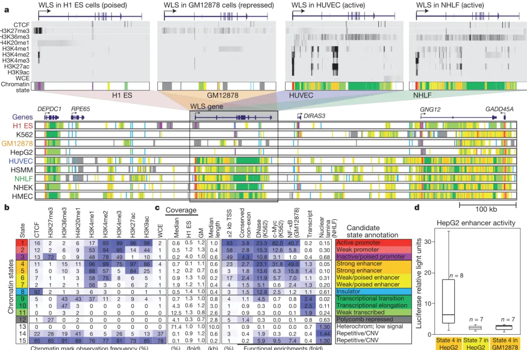
Learning a common set of chromatin states across cell types To summarize these data sets into nine readily interpretable annota-tions, one per cell type, we applied a multivariate hidden Markov model that uses combinatorial patterns of chromatin marks to distin-guish chromatin states8. The approach explicitly models mark
com-binations in a set of ‘emission’ parameters and spatial relationships between neighbouring genomic segments in a set of ‘transition’ para-meters (Methods). It has the advantage of capturing regulatory ele-ments with greater reliability, robustness and precision than is possible by studying individual marks8.
We learned chromatin states jointly by creating a virtual conca-tenation of all chromosomes from all cell types. We selected 15 states that showed distinct biological enrichments and were consistently recovered (Fig. 1a, b and Supplementary Fig. 1). Even though states
were learned de novo solely on the basis of the patterns of chromatin marks and their spatial relationships, they showed distinct associa-tions with transcriptional start sites (TSSs), transcripts, evolutionarily conserved non-coding regions, DNase hypersensitive sites12, binding
sites for the regulators c-Myc13 (MYC) and NF-kB14, and inactive
genomic regions associated with the nuclear lamina15(Fig. 1c).
We distinguished six broad classes of chromatin states, which we refer to as promoter, enhancer, insulator, transcribed, repressed and inactive states (Fig. 1c). Within them, active, weak and poised4
promo-ters (states 1–3) differ in expression level, strong and weak candidate enhancers (states 4–7) differ in expression of proximal genes, and strongly and weakly transcribed regions (states 9–11) also differ in their positional enrichments along transcripts. Similarly, Polycomb-repressed regions (state 12) differ from heterochromatic and repetitive states (states 13–15), which are also enriched for H3K9me3 (Sup-plementary Figs 2–4).
The states vary widely in their average segment length (,500 base pairs (bp) for promoter and enhancer states versus 10 kb for inactive
0 10 20 30
Luciferase relative light units
b c d
a
Chromatin mark observation frequency (%) (%) (fold) (kb) (%) Functional enrichments (fold)
Candidate state annotation
CTCF
State H3K27me3 H3K36me3 H4K20me1 H3K4me1 H3K4me2 H3K4me3 H3K27ac H3K9ac WCE Median Median length ±2 kb TSS Conserved non-exon DNase (K562) c-Myc (K562)
NF-κB
(GM12878) Transcript Nuclear lamina
HepG2 enhancer activity Coverage H1 ES GM 16 2 2 6 17 93 99 96 98 2 0.6 1.0 83 3.8 23.3 82.0 40.7 0.2 0.15 12 2 6 9 53 94 95 14 44 1 0.5 0.4 58 2.8 15.3 12.6 5.8 0.6 0.30 13 72 0 9 48 78 49 1 10 1 0.2 0.6 49 4.3 10.8 3.1 1.0 0.4 0.68 11 1 15 11 96 99 75 97 86 4 0.7 0.6 23 2.7 23.1 31.8 49.0 1.3 0.05 5 0 10 3 88 57 5 84 25 1 1.2 0.6 3 1.8 13.6 6.3 15.8 1.4 0.10 7 1 1 3 58 75 8 6 5 1 0.9 0.2 17 2.4 11.9 5.7 7.0 1.1 0.31 2 1 2 1 56 3 0 6 2 1 1.9 0.4 4 1.5 5.1 0.6 2.4 1.3 0.20 92 2 1 3 6 3 0 0 1 1 0.5 0.4 3 1.5 12.8 2.5 1.2 1.1 0.61 5 0 43 43 37 11 2 9 4 1 0.7 0.8 4 1.1 4.5 0.7 0.8 2.4 0.02 1 0 47 3 0 0 0 0 0 1 4.3 3.0 1 0.9 0.3 0.0 0.0 2.5 0.11 0 0 3 2 0 0 0 0 0 0 12.5 2.6 2 0.9 0.3 0.0 0.1 1.9 0.24 1 27 0 2 0 0 0 0 0 0 4.1 2.8 5 1.4 0.3 0.0 0.1 0.8 0.63 0 0 0 0 0 0 0 0 0 0 71.4 10.0 1 0.9 0.1 0.0 0.0 0.7 1.30 22 28 19 41 6 5 26 5 13 37 0.1 0.6 3 0.4 1.9 0.3 0.2 0.4 1.44 85 85 91 88 76 77 91 73 85 78 0.1 0.2 1 0.2 5.9 9.5 7.4 0.4 1.30 Active promoter Weak promoter Inactive/poised promoter Strong enhancer Strong enhancer Weak/poised enhancer Weak/poised enhancer Insulator Transcriptional transition Transcriptional elongation Weak transcribed Polycomb repressed Heterochrom; low signal Repetitive/CNV Repetitive/CNV 1 2 3 4 5 6 7 8 9 10 11 12 13 14 15 State 4 in
HepG2 State 7 inHepG2 GM12878State 4 in
0.5 1.2 1.2 1.3 4.0 1.0 0.1 1.1 0.2 0.7 1.3 1.0 1.2 1.1 1.4 1.0 1.3 1.0 0.6 1.2 1.3 0.8 0.3 0.7 1.0 1.0 0.9 1.2 0.9 1.0 H1 ES K562 GM12878 HepG2 HUVEC HSMM NHLF NHEK HMEC Genes GM12878 H1 ES CTCF H3K27me3 H3K36me3 H4K20me1 H3K4me1 H3K4me2 H3K4me3 H3K27ac H3K9ac WCE Chromatin state Chromatin states WLS gene DIRAS3 GNG12 GADD45A
WLS in H1 ES cells (poised) WLS in GM12878 cells (repressed) WLS in HUVEC (active) WLS in NHLF (active)
RPE65 DEPDC1 HUVEC NHLF 100 kb n = 7 n = 7 n = 8 (NHLF)
Figure 1|Chromatin state discovery and characterization. a, Top: profiles for nine chromatin marks (greyscale) are shown across the WLS gene in four cell types, and summarized in a single chromatin state annotation track for each (coloured according to b). WLS is poised in ESCs, repressed in GM12878 and transcribed in HUVEC and NHLF. Its TSS switches accordingly between poised (purple), repressed (grey) and active (red) promoter states; enhancer regions within the gene body become activated (orange, yellow); and its gene body changes from low signal (white) to transcribed (green). These chromatin state changes summarize coordinated changes in many chromatin marks; for example, H3K27me3, H3K4me3 and H3K4me2 jointly mark a poised
promoter, whereas loss of H3K27me3 and gain of H3K27ac and H3K9ac mark promoter activation. WCE, whole-cell extract. Bottom: nine chromatin state tracks, one per cell type, in a 900-kb region centred at WLS, summarizing 90 chromatin tracks in directly interpretable dynamic annotations and showing activation and repression patterns for six genes and hundreds of regulatory regions, including enhancer states. b, Chromatin states learned jointly across
cell types by a multivariate hidden Markov model. The table shows emission parameters learned de novo on the basis of genome-wide recurrent
combinations of chromatin marks. Each entry denotes the frequency with which a given mark is found at genomic positions corresponding to the chromatin state. c, Genome coverage, functional enrichments and candidate annotations for each chromatin state. Blue shading indicates intensity, scaled by column. CNV, copy number variation; GM, GM12878. d, Box plots depicting enhancer activity for predicted regulatory elements. Sequences 250 bp long corresponding either to strong or weak/poised HepG2 enhancer elements or to GM12878-specific strong enhancer elements were inserted upstream of a luciferase gene and transfected into HepG2. Reporter activity was measured in relative light units. Robust activity is seen for strong enhancers in the matched cell type, but not for weak/poised enhancers or for strong enhancers specific to a different cell type. Boxes indicate 25th, 50th and 75th percentiles, and whiskers indicate 5th and 95th percentiles.
RESEARCH
ARTICLE
4 4 | N A T U R E | V O L 4 7 3 | 5 M A Y 2 0 1 1
Macmillan Publishers Limited. All rights reserved ©2011
to target genes. Investigation of four recent quantitative trait locus studies in liver20 and lymphoblastoid cells21–23 revealed remarkable
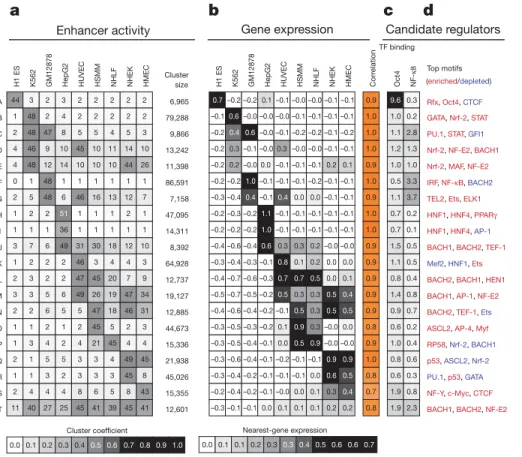
agreement with our enhancer predictions. Enhancers linked to a given target gene by our method were significantly enriched for SNPs cor-related with the gene’s expression level (Supplementary Fig. 17), thus confirming our enhancer–gene linkages with orthogonal data. Correlations with transcription factor expression and motif enrichment predict upstream regulators
We next predicted, on the basis of regulatory motif enrichments, sequence-specific transcription factors likely to target enhancers in a given cluster. This implicated a number of transcription factors whose known biological roles matched the respective cell types (Fig. 3d and Supplementary Fig. 18). When ChIP-seq data on the relevant cell type was available, we confirmed that enriched motifs were preferentially bound by the cognate factor (Fig. 3c). Oct4 (POU5F1) motif instances in cluster A (ESC-specific enhancers) were preferentially bound by Oct4 in ESCs24, and NF-kB motif instances in
cluster F (lymphoblastoid-specific enhancers) were preferentially bound by NF-kB in lymphoblastoid cells14. In both cases, motif
instances in cell-type-specific enhancers showed a ,5-fold increase in binding in comparison with other enhancers.
However, sequence-based motif enrichments do not distinguish causality. Enrichment could reflect a parallel binding event that does not affect the chromatin state, or the motif could actually be antagonistic to the enhancer state through specific repression in orthogonal cell types. To distinguish between these possibilities, we complemented the observed motif enrichments with cell-type-specific expression for the corresponding transcription factors (Fig. 3e). We then correlated a ‘motif score’ based on motif enrichment in a given cluster, and a ‘transcription factor expression score’ based on the agreement between
the transcription factor expression pattern and the cluster activity pro-file (Methods). A positive correlation between the two scores implies that the transcription factor may be establishing or reinforcing the chromatin state. A negative correlation would instead imply that the transcription factor may act as a repressor. For example, in addition to the enrichment of the Oct4 motif in the ESC-specific cluster A, Oct4 is specifically expressed in ESCs, leading to the prediction that it is a causal regulator of ESCs (Fig. 3e), consistent with known biology16.
For 18 of the 20 clusters, this analysis revealed one or more can-didate regulators. Recovery of known roles for well-studied regulators validated our approach. For example, HNF1 (HNF1A), HNF4 (HNF4A) and PPARc (PPARG) are predicted as activators of HepG2-specific enhancers (clusters H and I), PU.1 (SPI1) and NF-kB as activators of lymphoblastoid (GM12878) enhancers (clusters C, F and G), GATA1 as an activator of K562-specific enhancers (cluster B) and Myf family members as HSMM enhancers14,25–27 (cluster O).
The analysis also revealed potentially novel regulatory interactions. ETS-related factors (ELK1, TEL2 (ETV7) and Ets family members) are predicted activators of enhancers active in both GM12878 and HUVEC (cluster G) but not of GM12878-specific or HUVEC-specific clusters, emphasizing the value of unbiased clustering. These connec-tions are consistent with reported roles for ETS factors in lympho-poiesis and endothelium28. The prediction of p53 (TP53) as an
activator in HSMM, NHLF, NHEK and HMEC (clusters N, Q and R) probably reflects its maintained activity in these primary cells, as opposed to cell models in which it may be suppressed by mutation (K562)29, viral inactivation (GM12878)30or cytoplasmic localization
(ESCs)31. A widespread role for p53 in regulating distal elements is
consistent with its known binding to distal regions32,33.
Our analysis also revealed several repressor signatures, including GFI1 in K562 and GM12878 (clusters B and C) and BACH2 in ESCs
a Enhancer activity b Gene expression c Candidate regulators d e
Activator/repressor activity signatures
A A B B C C D D E E F F G G H H I I J J K K L L M M N N O O P P Q Q R R S S T T
H1 ES K562 GM12878 HepG2 HUVEC HSMM NHLF NHEK HMEC size Cluster
H1 ES K562 GM12878 HepG2 HUVEC HSMM NHLF NHEK HMEC Corr
elation
Oct4
NF-κB
TF binding
Top motifs Oct4 Rfx GATA PU.1 STAT NF-E2 NF-κB IRF ELK1 TEL2 Ets HNF1 HNF4 PPAR
γ
TEF-1 Myf RP58 p53 c-Myc Mef2 AP-1 MAF BACH1 GFI1 BACH2 CTCF AP-4 NF-Y HEN1 Nrf-2 ASCL2 44 3 2 3 2 2 2 2 2 6,965 0.7–0.2 –0.2 0.1 –0.1 –0.0 –0.0 –0.1 –0.1 0.9 9.6 0.3
(enriched/depleted)
1 48 2 4 2 2 2 2 2 79,288 –0.10.6–0.0 –0.0 –0.0 –0.1 –0.1 –0.1 –0.1 1.0 1.0 0.2 GATA, Nrf-2, STAT Rfx, Oct4, CTCF
2 48 47 8 5 5 4 5 3 9,866 –0.20.4 0.6–0.0 –0.1 –0.2 –0.2 –0.1 –0.2 1.0 1.1 2.8 PU.1, STAT, GFI1 4 46 9 10 45 10 11 14 10 13,242 –0.2 0.3 –0.1 –0.0 0.3 –0.0 –0.0 –0.1 –0.1 1.0 1.2 1.3 Nrf-2, NF-E2, BACH1
4 48 12 14 10 10 10 44 26 11,398 –0.2 0.2 –0.0 0.0 –0.1 –0.1 –0.1 0.2 0.1 0.9 1.0 1.0 Nrf-2, MAF, NF-E2
0 1 48 1 1 1 1 1 1 86,591 –0.2 –0.21.0–0.1 –0.1 –0.1 –0.2 –0.1 –0.1 1.0 0.5 3.3 IRF, NF-κB, BACH2 2 5 48 6 46 16 13 12 7 7,158 –0.3 –0.40.4–0.10.4 0.0 0.0 –0.1 –0.1 0.9 1.1 3.7 TEL2, Ets, ELK1
1 2 2 51 1 1 1 2 1 47,095 –0.2 –0.3 –0.21.1–0.1 –0.1 –0.1 –0.1 –0.1 1.0 0.7 0.2 HNF1, HNF4, PPARγ
1 1 1 36 1 1 1 1 1 14,311 –0.2 –0.2 –0.21.0–0.1 –0.1 –0.1 –0.1 –0.1 1.0 0.7 0.1 HNF1, HNF4, AP-1 3 7 6 49 31 30 18 12 10 8,392 –0.4 –0.6 –0.40.6 0.3 0.3 0.2 –0.0 –0.0 0.9 1.5 0.5 BACH1, BACH2, TEF-1
1 2 2 2 46 3 4 4 3 64,928 –0.3 –0.4 –0.3 –0.10.8 0.1 0.2 0.0 0.0 0.9 1.1 0.5 Mef2, HNF1, Ets
2 3 2 2 47 45 20 7 9 12,737 –0.4 –0.7 –0.6 –0.30.7 0.7 0.5 0.0 0.1 0.9 0.8 0.4 BACH2, BACH1, HEN1
3 3 5 6 49 26 19 47 34 19,127 –0.5 –0.7 –0.5 –0.20.5 0.3 0.3 0.5 0.4 0.9 1.4 0.8 BACH1, AP-1, NF-E2
2 2 6 5 5 47 18 46 31 12,885 –0.4 –0.6 –0.4 –0.2 –0.10.5 0.3 0.5 0.5 0.9 0.9 0.7 BACH2, TEF-1, Ets 1 1 2 1 2 45 5 2 3 44,673 –0.3 –0.5 –0.3 –0.2 0.1 0.9 0.3 –0.0 0.0 0.8 0.6 0.2 ASCL2, AP-4, Myf
1 3 4 2 4 21 45 4 4 15,336 –0.3 –0.5 –0.4 –0.1 0.0 0.5 0.9–0.0 –0.0 0.9 1.0 0.4 RP58, Nrf-2, BACH1 2 1 5 5 3 3 4 49 45 21,938 –0.3 –0.6 –0.4 –0.1 –0.2 –0.1 –0.10.9 0.9 1.0 0.8 0.6 p53, ASCL2, Nrf-2 1 1 3 2 3 3 3 45 8 45,026 –0.3 –0.4 –0.2 –0.1 –0.1 –0.1 0.0 0.6 0.5 0.8 0.6 0.3 PU.1, p53, GATA 2 4 4 4 8 6 5 8 43 15,355 –0.2 –0.4 –0.2 –0.1 –0.0 0.0 0.1 0.3 0.4 0.7 1.9 0.8 NF-Y, c-Myc, CTCF
11 40 27 25 45 41 39 45 41 12,601 –0.3 –0.1 –0.1 0.0 0.1 0.1 0.1 0.2 0.2 0.8 1.9 2.3 BACH1, BACH2, NF-E2
Cluster coefficient/gene expression correlation
–1.0 –0.8–0.6 –0.4 –0.2 0.0 0.2 0.4 0.6 0.8 1.0
Regulatory motif enrichment
–1.0 –0.8 –0.6–0.4 –0.2 0.0 0.2 0.4 0.60.8 1.0 TF expression –1.0 –0.8 –0.6 –0.4 –0.2 0.0 0.2 0.4 0.6 0.8 1.0 TF/motif correlation –1.0 –0.8–0.6 –0.4 –0.2 0.0 0.2 0.4 0.6 0.8 1.0 Cluster coefficient 0.0 0.1 0.2 0.3 0.4 0.5 0.6 0.7 0.8 0.9 1.0 Nearest-gene expression 0.0 0.1 0.1 0.2 0.3 0.3 0.4 0.5 0.6 0.6 0.7 Activator signature Positive correlation Motif enrichment/TF expression Motif depletion/TF repression
Repressor signature Negative correlation Motif depletion/TF expression Motif enrichment/TF repression
Figure 3|Correlations in activity patterns link enhancers to gene targets and upstream regulators. a, Average enhancer activity across the cell types (columns) for each enhancer cluster (rows) defined in Fig. 2b (labelled A–T) and number of 200-bp windows in each cluster. b, Average messenger RNA expression of nearest gene across the cell types and correlation with enhancer activity profile from a. High correlations between enhancer activity and gene expression provide a means of linking enhancers to target genes. c, Enrichment for Oct4 binding in ESCs24and NF-kB binding in lymphoblastoid cells14for each
cluster. TF, transcription factor. d, Strongly enriched (red) or depleted (blue) motifs for each cluster, from a catalogue of 323 consensus motifs. Rfx: Rfx family; Nrf-2: NFE2L2; STAT: STAT family; Ets: Ets family; Mef2: MEF2A and MYEF2;
Myf: Myf family; NF-Y: NFYA, NFYB and NFYC. e, Predicted causal regulators for each cluster based on positive (activators) or negative (repressors)
correlations between motif enrichment (top left triangles) and transcription factor expression (bottom right triangles). For example, the red–yellow combination indicates that Oct4 is a positive regulator of ESC-specific
enhancers, as its motif-based predicted targets are enriched (red upper triangle) for enhancers active in ESCs (cluster A), and the Oct4 gene is expressed specifically in ESCs, resulting in a positive transcription factor expression correlation (yellow triangle). Overall correlations between motif enrichment and transcription factor expression across all clusters denote predicted activators (positive correlation, orange) and repressors (negative correlation, purple).
RESEARCH
ARTICLE
4 6 | N A T U R E | V O L 4 7 3 | 5 M A Y 2 0 1 1
Macmillan Publishers Limited. All rights reserved ©2011