Fac t or s c ont r ol l i ng i nt er - c at c hm
ent var i at i on
of m
ean t r ans i t t i m
e w
i t h c ons i der at i on of
t em
por al var i abi l i t y
著者
M
a W
enc hao, Yam
anaka Ts ut om
u
j our nal or
publ i c at i on t i t l e
J our nal of hydr ol ogy
vol um
e
534
page r ange
193- 204
year
2016- 03
権利
( C) 2016. Thi s m
anus c r i pt ver s i on i s m
ade
avai l abl e under t he CC- BY- N
C- N
D
4. 0 l i c ens e
ht t p: / / c r eat i vec om
m
ons . or g/ l i c ens es / by- nc - nd/ 4
. 0/
U
RL
ht t p: / / hdl . handl e. net / 2241/ 00141475
doi: 10.1016/j.jhydrol.2015.12.061
1 / 42
1
Factors controlling inter-catchment variation of mean transit time with consideration of
2
temporal variability
3
4
Wenchao Ma and Tsutomu Yamanaka, Center for Research in Isotopes and Environmental Dynamics,
5
University of Tsukuba, Japan; Faculty of Life and Environmental Sciences, University of Tsukuba, Japan
6
7
Corresponding author:
8
Wenchao Ma E-mail: [email protected]
9
Phone: +81-29-852-2533
10
Address: 1-1-1 Tennoudai, Tsukuba, Japan
11
TsutomuYamanaka E-mail: [email protected]
12
Phone: +81-29-853-2538
13
Address: 1-1-1 Tennoudai, Tsukuba, Japan
14
15
16
Abstract: 17
The catchment transit time, a lumped descriptor reflecting both time scale and spatial structure of
18
catchment hydrology can provide useful insights into chemical/nuclear pollution risks within a catchment.
19
Despite its importance, factors controlling spatial variation of mean transit time (MTT) are not yet well
20
understood. In this study, we estimated time-variant MTTs for about ten years (2003–2012) in five
2 / 42
mesoscale sub-catchments of the Fuji River catchment, central Japan, to establish the factors controlling
22
their inter-catchment variation with consideration of temporal variability. For this purpose, we employed a
23
lumped hydrological model that was calibrated and validated by hydrometric and isotopic tracer
24
observations. Temporal variation patterns of estimated MTT were similar in all sub-catchments, but with
25
differing amplitudes. Inter-catchment variation of MTT was greater in dry periods than wet periods,
26
suggesting spatial variation of MTT is controlled by water ‘stock’ rather than by ‘flow’. Although the
27
long-term average MTT (LAMTT) in each catchment was correlated with mean slope, coverage of forest (or
28
conversely, other land use types), coverage of sand–shale conglomerate, and groundwater storage, the
29
multiple linear regression revealed that inter-catchment variation of LAMTT is principally controlled by the
30
amount of groundwater storage. This is smaller in mountainous areas covered mostly by forests and greater
31
in plain areas with less forest coverage and smaller slope. This study highlights the topographic control of
32
MTT via groundwater storage, which might be a more important factor in mesoscale catchments, including
33
both mountains and plains, rather than in smaller catchments dominated by mountainous topography.
34
35
Keywords: transit time; catchment hydrology; tank model; isotope tracer; Fuji River
36
37
1. Introduction 38
Given a scenario of a water pollution accident, such as that following a nuclear bomb, it is imperative to
39
know how long it would take the polluted water to reach any specific location, especially sources of
40
domestic water supply systems. The catchment transit time, which is defined as the elapsed time from when
41
a water molecule enters a catchment across the land surface until it exits at the catchment outlet through the
3 / 42
stream network (Bolin and Rodhe, 1973; McDonnell et al., 2010), has been one of the major research topics
43
in the field of catchment hydrology. It reflects the storage, flow pathway, and sources of water within the
44
catchment, in addition to how the catchment retains and releases water (McGuire and McDonnell, 2006).
45
Therefore, knowledge of the catchment transit time can provide useful insights with regard to taking prompt
46
appropriate measures against chemical/nuclear pollution events.
47
As the transit time differs for each individual water molecule, we have to consider the mean transit time
48
(MTT) and transit time distribution (TTD) for a mass of water molecules. In earlier works (Maloszewski and
49
Zuber, 1982; Maloszewski et al., 1983; DeWalle et al., 1997; Ozyurt and Bayari, 2003), MTT has usually
50
been estimated by modeling input–output relationships of conservative tracers such as stable isotopes or
51
chloride under the assumption of steady-state and using hypothetical TTD functions. These simple
52
treatments for estimating MTT have become controversial and new methods based on time-variant TTDs or
53
without an explicit form of TTD have been developed to estimate MTT (McGuire et al., 2002; Sayama and
54
McDonnell, 2009; Duffy, 2010; Ma and Yamanaka, 2013). These studies demonstrated that TTDs can
55
change rapidly over time and through responding to rainfall and drought events, they are highly irregular in
56
shape, which introduces considerable temporal variability to the MTT. Recently, other tracers were newly
57
applied to relative research destinations. Such as, nutrient was testified identifiable during hydrological and
58
biogeochemical responses (Hrachowitz et al., 2015), as well as Fovet et al., (2014) estimated the nitrogen
59
transit time in headwater catchment; Peters et al., (2014) combine used groundwater 3H/3He ages and
60
dissolved silica (Si) concentrations for investigating mean streamwater transit time; hexavalent chromium
61
(Cr(VI)) and chromium hydroxide (Cr(OH)3(s)) were used by Druhan and Maher (2014) in structurally
62
correlated subsurface heterogeneous porous media.
4 / 42
Hydrological variations are generally introduced by many factors such as climate, soil and soil water
64
transit time were carried out by Tetzlaff et al. (2014), Kim and Jung (2014), Stockinger et al., (2014), Timber
65
et al., (2015), vegetation, topography, geology, snow (Seeger and Weiler, 2014), and anthropogenic activities
66
(Blöschl, 2005). Therefore, catchment transit time is variable in space. Previous studies reported that MTT
67
depends upon topography (McGuire et al., 2005), soil (Soulsby et al., 2006a), or both (Soulsby et al., 2006b;
68
Tetzlaff et al., 2009; Hrachowitz et al., 2010). However, the correlation between MTT and catchment size
69
was not obvious, while inter-catchment variance of MTT decreased with increasing catchment size (Soulsby
70
et al., 2006a; Hrachowitz et al., 2010). Although these studies clarified the factors controlling transit time,
71
the temporal variabilities of MTT and TTD were not considered in their analyses and thus, the
72
understanding of the inter-catchment variation of time-variant MTT and its controlling factor(s) is
73
incomplete. McDonnell et al. (2010) stated as one of four research needs: “We need more work that relates
74
transit times to geographic, geomorphic, geologic, and biogeochemical characteristics of catchments.”
75
Stream MTTs in tropical montane regions (Muñoz-Villers et al., 2015), and temporal dynamics of catchment
76
transit times (Klaus et al., 2014) related to catchment characteristics were discussed, and both of these
77
researches were carried out in small catchment.
78
The objectives of the present study are to compare MTTs among catchments with consideration of their
79
temporal variability and to establish the factors controlling inter-catchment variation. A lumped hydrologic
80
model, which was calibrated/validated with hydrometric and isotopic measurements (Ma and Yamanaka,
81
2013) was employed for this purpose. Here, we focus on mesoscale catchments. Mesoscale catchments are
82
commonly associated with anthropogenic activities and thus, they are often of great interest regarding the
83
development of water resources and interventions intended to enhance rural livelihoods (Love et al., 2011).
84
Nevertheless, in mesoscale catchments, hydrological processes occurring on smaller scales develop in
5 / 42
complex ways to produce an integrated response (Scherrer and Naef, 2003; Uhlenbrook et al., 2004), such
86
that storm–runoff generation on the mesoscale has not yet been clarified. Therefore, studies on mesoscale
87
catchments are both significant and imperative.
88
89
2. Material and methods 90
2.1 Site description
91
The catchments investigated in this study are five sub-catchments (SCs) comprising the Fuji River
92
catchment (35.5–36.0°N, 138.2–138.9°E), central Japan (Fig. 1). The area of the total (i.e., Fuji River)
93
catchment is 2172.7 km2 and its elevation ranges from approximately 234.7 to 2962.8 m. Annual
94
precipitation is about 1135.2 mm, mean relative humidity is 65%, mean temperature is 14.7 °C, and the
95
mean wind speed is 2.2 ms−1 (based on records of meteorological observations between 1981 and 2010 at
96
Kofu station, operated by the Japan Meteorological Agency (JMA)). Northern, eastern, and western parts of
97
the catchment are characterized by mountainous topography, whereas the central and southern areas are
98
alluvial fans and lowlands. The mountains are formed mostly by granite and partly by andesitic/basaltic
99
rocks. The following geological compositions were found within the study area and taken into consideration:
100
basalt of undefined geological time (Ba), welded tuff of Quaternary age (Wt), sand–shale conglomerate of
101
Mesozoic age (Ss), and granite of undefined geological time (Gr). Forest is the dominant land-use type over
102
the entire study area with its percentage coverage ranging from 67% to 94%. The residual percentages are
103
mainly given over to agricultural land and range grassland. The land use/land cover is mainly formed by
104
forests in the mountainous areas, orchards and vegetable fields in the alluvial fans, and residential areas and
105
paddy fields in the alluvial lowlands. The five SCs were defined with consideration of the location of
6 / 42
gauging stations maintained by the Ministry of Land, Infrastructure, Transport, and Tourism.
107
108
2.2. Data
109
For the period from January 1, 2006 to September 30, 2012, AMeDAS (Automatic Meteorological Data
110
Acquisition System) radar precipitation data produced by the JMA were used to consider the spatial
111
variability of precipitation. These data provide maps of hourly accumulations of precipitation estimated from
112
combined observations from radars and rain gauges (e.g., see Makihara, 1996). The spatial resolution is
113
approximately 1 × 1 km. Before this period (i.e., 2003–2005), point precipitation data from
114
hydro-meteorological stations were used and the Thiessen polygon method applied to obtain areal mean
115
precipitation in each SC. The locations of the hydro-meteorological stations are shown in Fig. 1.
116
Data of observed daily river discharge produced by the Ministry of Land, Infrastructure, Transport, and
117
Tourism (MLIT) were used for each SC. For calculating the evapotranspiration, we applied the FAO
118
Penman–Monteith method (Allen et al., 1998). Meteorological data (solar radiation, air temperature, relative
119
humidity, and wind speed) observed by the JMA at three weather stations (Fig. 1) were used. Based on the
120
relationships between the elevation of the stations and the meteorological variables, representative values
121
were estimated considering the mean elevation of each SC, which were then used for the evapotranspiration
122
computation. Here, temperature was regressed considering elevation affect, around -0.57 °C difference of
123
100 meter elevation increased for the local catchment. For other meteorological parameters, we applied
124
values at a nearest station for the whole catchment. (Figure 1.)
125
In addition to the existing data set, we performed monthly isotopic monitoring of river water at the
126
Ministry of Land, Infrastructure, Transport, and Tourism gauging stations from April 2010 (or April 2011) to
7 / 42
March 2012. Monthly monitoring of the precipitation isotope was also performed at Kofu (Fig. 1). A
128
precipitation collector (Shimada et al., 1992, Yamanaka et al., 2004) that can prevent the evaporation of
129
stored precipitation was used for collecting monthly precipitation, and the mixed value representing average
130
of precipitation isotope composition for the relative month (Ma and Yamanaka, 2013). Hydrogen and
131
oxygen stable isotope ratios (2H/1H and 18O/16O) of the collected water samples were measured using a
132
tunable diode laser isotope analyzer (L11020-I, Picarro, CA, USA). The measurement errors for this
133
analyzer were 0.1‰ for δ18O and 1‰ for δD (Yamanaka and Onda, 2011). For each SC, the mean values of
134
δ18O and δD of precipitation were estimated considering regional altitudinal effects (1.6‰/100 m for δ18O
135
and 6.4‰/100 m for δD), which were determined from the data set of Makino(2013).
136
137
3. Theory 138
The lumped hydrologic model for estimating time-variant MTT (and TTD) has been successfully applied
139
in the Fuefuki River catchment (Ma and Yamanaka, 2013). However, the applicability of this model to other
140
catchments is still unknown; therefore, in this study, we applied it to the five SCs of the Fuji River
141
catchment, which includes the Fuefuki River catchment (SC3). The detailed equations of this tracer-aided
142
tank model were not provided in the main text of Ma and Yamanaka (2013); therefore, we outline the
143
principal specific steps here.
144
3.1 Water balance
145
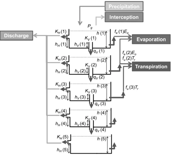
The model is composed of five tanks in series vertically, where the water flow within each conceptually
146
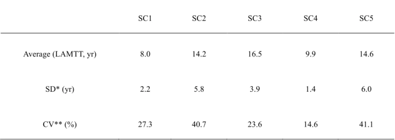
represents the overland flow, rapid throughflow, delayed throughflow, groundwater flow, and in-bedrock
147
flow, respectively (Fig. 2). The model was initialized by spin-up with the initial two years data. Total runoff
8 / 42
Q, horizontal water flux (strictly, towards a stream network) [qH(i)), and vertical water flux [qV(i)] for the
149
i-th tank can be computed by the following equations in daily steps, respectively:
150 5 1 ( ) H i
Q q i
=
=
∑
(1)151
( )
(
)
( ) max ( ) ( ) , 0
H H H
q i = ⎡⎣k i h i −h i ⎤⎦, (2)
152
( )
(
)
( ) max ( ) ( ) , 0
V V V
q i = ⎡⎣k i h i −h i ⎤⎦, (3)
153
where h(i) is the water level in the i-th tank, hV(i) is the level of the top of the vertical pipes connecting the
154
bottom outlets, hH(i) is the level of the lateral outlets, and kV(i) and kH(i) are the conductance parameters
155
analogous to the hydraulic coefficients of Darcy’s law, which regulate qV(i) and qH(i), respectively.
156
Furthermore, the differences between h(i) and hV(i) or hH(i) correspond to the hydraulic gradient. The
157
magnitude of ΔhH-V [≡hH(i) − hV(i); > 0, in normal cases] controls the relative importance of the horizontal
158
and vertical flows within each layer, such that the values of kV(i), kH(i), and ΔhH-V are determined through 159
calibration based on the comparison of the observed and predicted hydrographs.
160
One of the simplifications in this method is that water level (i.e., analogous to potential) in a lower tank
161
does not affect flow from an upper tank and that the flow direction is always downward. This permits the
162
avoidance of an iteration procedure in computing fluxes and potentials and thus, the computation time can
163
be reduced markedly. Similarly, for the horizontal fluxes (or runoff components), water level in a stream
164
channel is not considered, and the scale of the distance between the stream channel and a point at which the
165
hydraulic status is represented by the water level in the tank is unknown. This vague expression does
166
introduce uncertainties, mainly in the determination of conductance parameters kH(i), but it might implicitly
167
represent the variable source area concept.
168
Water budget equations for the 1st and the other four tanks are given as follows, respectively:
9 / 42
dh i( ) P I f i TT( ) r f i EE( ) S q iV( ) qH( ) for =1i i
dt = − − − − − , (4) 170
( )
( 1) ( ) ( ) ( ) ( ) for =2-5
V T r E S V H
dh i
q i f i T f i E q i q i i
dt = − − − − − , (5)
171
where t is time, P is precipitation, I is interception loss, Tr is transpiration, Es is soil evaporation, and fT(i)
172
and fE(i) are weighting factors at the i-th tank for root water uptake and soil evaporation, respectively. We
173
assume I = fIP, and the fI value were set as 0.164, 0.133, 0.118, 0.117 and 0.151 for each catchment
174
considering the percentage of land use and vegetation, and the ratios following previous work on humid
175
temperate forests (Sugita and Tanaka, 2009). Evapotranspiration, ET (= Tr + Es + I), is estimated as
176
, (6)
177
where Kc is the single-crop coefficient and ETo is the reference evapotranspiration obtained from the FAO
178
Penman–Monteith equation (Allen et al., 1998). We applied the value of Kc (= 1) for conifer trees.
179
According to Kubota and Tsuboyama (2004), the proportion of soil evaporation to total evapotranspiration
180
in forests generally ranges from 3% to 20% with an average of 10%. Thus, we assign Es and Tr as follows:
181
, (7)
182
, (8)
183
where FE (=0.1 in the present study) is Es/ET. In forests in central Japan, the zone of root water uptake is
184
usually <50 cm beneath the ground surface, although some species do take up water from soil at depths >1
185
m (Yamanaka et al., 2009). Therefore, we assumed fT(1, 2, 3, 4, 5) = (0, 0.7, 0.3, 0, 0). In addition, we
186
assumed that soil evaporation does not occur in the deeper tanks, i.e., fE(3, 4, 5) = (0, 0, 0). The values for
187
fE(i) in the shallower tanks depend on the amount of water in the tank, as follows:
188
10 / 42
fE
( )
1 =1 for h
( )
1 t>00 for h
( )
1t≤0 "# $
%$
, (9)
190
fE
( )
2 =1 for h
( )
2 t >00 for h
( )
2 t≤0 "# $
%$
, (10)
191
where superscript “t” means the value for the subsequent time step.
192
Although fT(i), fE(i), fI(i), Kc(i), and FE(i) should depend on land use type and/or vegetation condition, we
193
set the values for typical forests within the study area because forest is the most dominant land cover within
194
most of the studied catchments.
195
3.2 Isotope balance
196
For the water balance calculation, water fluxes are decided by h(i) − hH(i) and h(i) − hV(i), as shown by
197
equations (2) and (3). This means that only the value hH(i)−hV(i) can be calibrated by hydrographs, and the
198
absolute values of hH(i) and hV(i) cannot been fixed. However, isotope data allows for calibrating them,
199
because concentration of tracers depends on absolute volume of water reservoir rather than on hydraulic
200
gradient. In other words, use of hydrograph alone (without isotopes) cannot constrain tank parameters,
201
providing worse estimates of MTT. The values of hV(i) or hH(i) also regulate isotope mixing within each tank,
202
as described below. This is the reason why we modeled not only water balance, but also isotope balance. The
203
isotopic composition is assumed to well mixed instantaneously within each tank.
204
Referring to the relevant water balance component, the isotopic composition of total runoff δQ can be
205 obtained as: 206
( )
( )
5 1 H w i Qq i i
Q δ
δ =
∑
= , (11)207
where δ is the isotopic composition (i.e., δ18O or δD) and values of hV(i) are determined by comparing the
11 / 42
predicted and observed δQ. In the type of tank model commonly used for predicting only runoff, hV(i) = 0 is
209
assumed. Determination hV(i) is less sensitive to hydrograph, but more sensitive to isotopic tracers.
210
The isotope budget equation in each tank is expressed as follows:
211
( )
(
)
[
]
( )
( )
( ) ( ) ( ) ( ) for =1
w
P T r V H w E S E
dh i i
P I f i T q i q i i f i E i
dt δ
δ δ δ
= − − + + − , (12)
212
( )
[
]
( )
( )
( 1) ( ) ( ) ( ) ( ) for =2-5
w
V P T r V H w E S E
dh i i
q i f i T q i q i i f i E i
dt δ
δ δ δ
= − − + + − , (13)
213
where subscripts P, E, and w denote precipitation, soil evaporation, and water, respectively, in each tank.
214
Instantaneous and complete mixing within each tank is assumed in this model. The value of δE can be
215
obtained by the following Craig–Gordon model (Craig and Gordon, 1965; Gat et al., 1996), and the kinetic
216
fractionation Δε is defined as:
217
( )
(
)
33 1 1 10
for =1 or 2
1 10
w a a
E
a
i h
i h
δ α δ α ε
δ
ε
− − − × − Δ
=
− +Δ , (14) 218
(
)
(
)
31 M n 1 10
a i
h ρ D D
ε
ρ ⎡ ⎤
Δ = − ⎣ − ×⎦ , (15)
219
where α is the equilibrium isotopic fractionation factor as a function of temperature (for experimental
220
functions, see Majoube (1971)), ha is the relative humidity of air, and δa is the isotopic composition of
221
atmospheric water vapor. The parameter ρM, is the resistance to molecular diffusion of water vapor, ρ is the
222
total resistance to water vapor transfer from the evaporating surface to the air, D is the water vapor
223
diffusivity in the air, Di is the water vapor diffusivity for heavy isotopes, and n is a semi-empirical parameter
224
(=1/2 for fully turbulent conditions). According to the experimental results of Cappa et al. (2003), D/Di is
225
equal to 1.0319 for oxygen and 1.0164 for hydrogen. A representative value of ρM/ρ is 0.32 (Yamanaka,
226
2009). Strictly, ha is the vapor pressure normalized by the saturation vapor pressure at the temperature of the
227
evaporating surface rather than air temperature; however, we used relative humidity in the common sense
12 / 42
for convenience.
229
After the values of hV(i) or hH(i) were determined, the storage of each layer of each SC was calculated as
230
the thickness of each tank; thus, total storage was considered as the sum of the storage over all the layers.
231
3.3 Calibration and validation
232
Calibrations of the model parameters were made considering the Nash–Sutcliffe Efficiency (NSE) for
233
water balance. The NSE is a normalized statistic that determines the relative magnitude of the residual
234
variance (“noise”) compared with the measured data variance (“information”) (Nash and Sutcliffe, 1970),
235
and it is represented by the following equation:
236
(
)
2(
)
21 1
1 /
n n
obs sim obs mean
i i i i
i i
NSE Y Y Y Y
= =
⎡ ⎤
= −⎢ − − ⎥
⎣
∑
∑
⎦, (16)
237
where Y is the runoff, and super scripts obs, sim, and mean denote the observed, simulated, and mean values,
238
respectively. For isotope balance, the root mean square error (RMSE) rather than NSE was used for
239
calibration, because the measured data variance of river water isotopic composition is very small. The NSE
240
was used for calibrating kH,kV, and ΔhH-V, and then the RMSE was used for hH (and thus, hV).
241
To obtain the optimal combination of values of the model parameters, the Monte Carlo simulation was
242
employed. This method performs random sampling of parameter values from a possible range, followed by
243
model evaluations using NSE and RMSE for a set of the sampled values. The possible range was set to be
244
±5% around the newest optimal value for each parameter in the iteration calculations. In the procedure of
245
calibration for isotope balance, the combined-RMSE (≡{RMSEδD/8 + RMSEδ18O}/2) was used for selecting
246
the best parameter set for both δ18O and δD, because a set of parameters providing the best result for δ18O is
247
not always the best for δD, and vice versa. The contribution of δD was divided by 8, according to theory of
248
GMWL, and the average value were used for representing combined use of δ18O and δD. Here we used
13 / 42
RMSE rather than NSE as a measure of model performance, because variation range of isotopic data is
250
relatively small and thus NSE was too sensitive.
251
After the calibration, model validation was performed for a period different to the calibration period.
252
Model performance in the validation was represented by NSE for water balance and RMSE for isotope
253
balance, as well as in the calibration.
254
3.4 Estimation of time-variant MTT
255
To estimate time-variant MTT using a calibrated/validated tank model, a virtual (or imaginary) “age”
256
tracer was introduced into the model (such an approach has been attempted previously by Goode (1996)for
257
groundwater and Khatiwala et al.(2001)for oceans).
258
If we define the age as the time elapsed from the water entering the catchment across the ground surface,
259
then A(1) = 0 throughout the simulation period. Solving A(i) under this boundary condition means that the
260
value of A(i) indicates the mean age of the water in each tank and therefore, MTT (AQ) can be predicted as:
261
( ) ( )
5 1 H i Qq i A i
A
Q =
=
∑
, (17)
262
where, if we take a time step of one day, the units of A(i) and AQ are days, and the final term, which is unity,
263
indicates the rate of ageing (Fig. 2). The concentration of this conservative and non-reactive tracer A(i) is
264
computed by
265
266
ΔA i
( )
=qV i−1
(
)
A i(
−1)
dt− qV
( )
i +qH( )
i +fTTr+fEES(
)
A i( )
dth i
( )
+1 for i=2-5. (18)
267
14 / 42 4. Results and discussion
269
4.1 Water and isotope balance
270
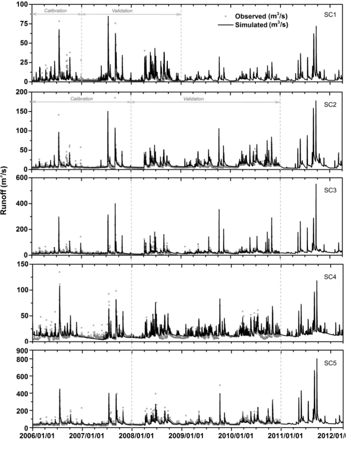
The simulated discharge largely agrees with that observed (Fig. 3), although a few discrepancies exist.
271
For example, some peaks of observed discharge could not be reproduced or were underestimated in the
272
simulation, especially for SC1 and SC2 in 2006, SC3 in 2006 and 2009, SC4 in 2006–2007, and SC5 in
273
2006 and 2008. These discrepancies might be attributable to inaccuracies in the precipitation data used in
274
the simulation, because the study catchments are mountainous with relatively large extent, such that the
275
spatial distribution of precipitation is highly heterogeneous and difficult to observe accurately.
276
Overestimations of discharge peaks (e.g., for all SCs in late 2009, SC1 in 2008, and SC3 in 2010) could
277
also be attributed to the same cause. Conversely, underestimations (e.g., SC1, SC3, and SC4 in 2007) and
278
overestimations (e.g., SC4 in 2008 and 2010) of simulated discharge in low flow periods seem to be
279
introduced by errors not just in precipitation, but also evapotranspiration. In the simulation,
280
hydro-meteorological data observed at a few stations were used, such that it is difficult to represent
281
precisely the fields of temperature, wind speed, and solar radiation for the entire catchment.
282
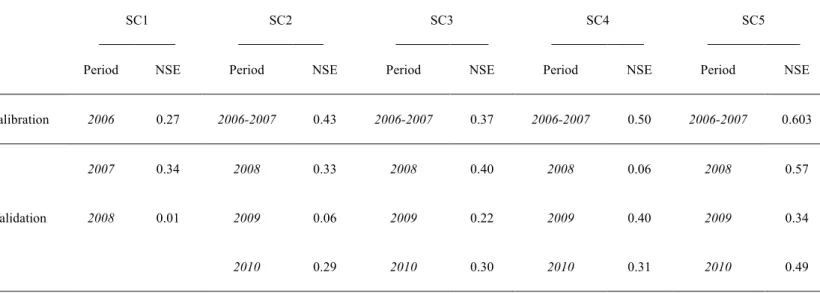
According to Moriasi et al. (2007), simulation results can be considered satisfactory if NSE is more
283
than 0.36. In our results, NSE ranges from 0.3 to 0.6 in most cases, although those for SC1 and SC4 in
284
2008 and for SC3 in 2009 are less than 0.1 (Table 1). And, the ratio of simulated runoff compare observed
285
ones are around 88.7% for the five catchments. Low performance in these specific cases is probably
286
associated with inaccuracies in the precipitation data and evapotranspiration estimations. It is undeniable
287
that limitation exist for a lumped model to reproduce these entire events precisely, especially for
288
meso-scale catchment with complicated characters on daily step. However, the model used in this study is
15 / 42
shown capable of reproducing the water balance in all five SCs reasonably well.
290
A water balance simulation or simulated discharge is closely related to the ‘change’ in water storage, but
291
is less sensitive to the water storage itself. However, an isotope balance simulation is closely related and
292
thus more sensitive to the absolute value of water storage. Therefore, better performance of an isotope
293
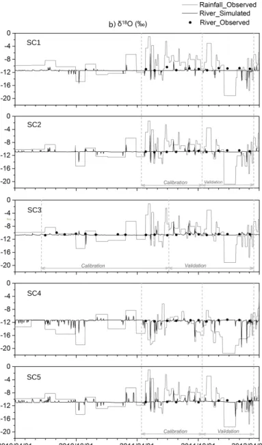
balance simulation can be linked to better estimation of transit time. Generally, the model in this study
294
reproduced well both δ18O and δD of river water in the five SCs (Fig. 4). However, as in water balance
295
simulation, both overestimations and underestimations can be found. One possible reason for the lower
296
isotope ratios in winter for some catchments might be snow melting, which was not considered in this
297
model. Also, rough estimations of evaporation and transpiration might be another reason. Relatively large
298
differences between the observed and simulated values exist, especially in the winter of 2011–2012
299
(excluding SC4), which might be caused by the spatial heterogeneity of precipitation isotope data. For the
300
simulations, precipitation isotope data were obtained only at the Kofu site and were corrected considering
301
catchment mean elevation, although spatial heterogeneity caused by factors other than elevation was not
302
considered. Thus, this could in part be the cause of the observation–simulation differences.
303
The RMSE ranges from 0.17–1.17‰ for δ18O and from 1.1–8.8‰ for δD (Table 1b). Surprisingly, the
304
RMSE is smaller in the validation than in the calibration, suggesting that the model used is valid, but that
305
its performance depends on the inter-annual changes in hydro-meteorological and/or isotopic conditions. In
306
the case of validation, the RMSE of δ18O (δD) is not greater than 0.57‰ (3.6‰). As the measurement error
307
of δ18O (δD) is 0.1‰ (1‰), as mentioned before, the isotope balance simulation in this study can be
308
regarded as acceptable. Unfortunately, because the temporal resolution of isotope monitoring in this study
309
is one month, the reproducibility of isotope variability in river water over shorter timescales is not
310
sufficiently validated. If isotope data with greater temporal resolution were used, the accuracy of the model
16 / 42
might be improved further. Snow coverage and melting processes were not considered in this model,
312
because the areal fraction of snow coverage is very small and yearly varied. Although there is an
313
undeniable isotopic effect caused by snow melting, especially for the winter and early spring river isotopic
314
composition, the influence is expected to be limited in considering with amounts of river water and
315
snowmelt water.
316
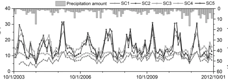
4.2 Temporal variation of MTT and its precipitation dependence
317
Fig. 5 represents the MTT variations for SC1–SC5 with total catchment average precipitation for about
318
ten years. While the MTT was originally computed in daily time steps, monthly averages are shown in this
319
figure. The monthly average MTT ranges from several years to decades; the variation range, as well as the
320
long-term average of MTT (LAMTT), differ for each SC (Table 2). The standard deviation (SD) and
321
coefficient of variation (CV) are lowest in SC4 and highest in SC2 and SC5. And, LAMTT is lowest in
322
SC1 (8.0 y) and highest in SC3 (16.5 y). The temporal variation patterns of MTT are similar among all the
323
SCs. As the precipitation amount increases, the MTT becomes smaller; high values of MTT can be found
324
during relatively dry periods. The annual cycle of MTT variation is clear, reflecting the seasonal variation
325
of precipitation amount.
326
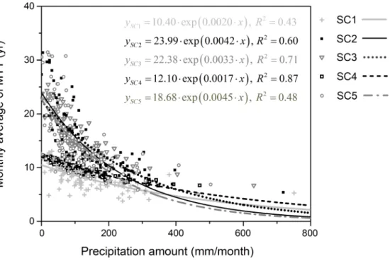
An inverse relationship between MTT and precipitation amount is clearly shown in Fig. 6. The
327
determination coefficients (R2) of the regression curves range from 0.43 (SC1) to 0.87 (SC4). The MTT
328
values are almost the same for all SCs when the amount of monthly precipitation is large, while
329
inter-catchment variation of MTT is exaggerated in dry periods. In other words, large storm events (i.e., high
330
flow conditions), which introduce new water with the same age, tend to erase or weaken inter-catchment
331
variation of MTT. Exponential regression was chosen for the better fitness than other regressions. However,
17 / 42
the equation does not provide enough matches for the large precipitations, which event account for less
333
percentage. One possible reason for this behavior might because that, processes and forming mechanism of
334
extreme precipitations, and the responses of catchments are different with normal precipitations.
335
4.3 Spatial variation of MTT and its controlling factors
336
As mentioned in the previous section, the temporal variation of MTT is caused mainly by precipitation,
337
and the dependence of MTT on precipitation differs for each SC. Thus, it is worth investigating which
338
factor(s) controls the spatial (i.e., inter-catchment) variability of MTT. Table 3 summarizes the correlations
339
between LAMTT and the potential controlling factors: area (i.e., catchment size), topography, geology, land
340
use/cover, and soil. As water storage within the catchment is expected to control MTT (especially for its
341
inter-catchment variation), the water storage volume in each layer of the tank is also added as a potential
342
factor. The correlation coefficient (R) is relatively high for the storage of Layer 4 (0.93), coverage of range
343
grass (0.91), coverage of forest (−0.89), coverage of agriculture (0.79), coverage of Ss (sand–shale
344
conglomerate of Mesozoic age; 0.80), and tangent of mean slope (−0.67). Fig. 7 displays scatter plots of
345
LAMTT versus selected factors. In this figure, range grass and agriculture were excluded, because their
346
percentages were relatively small and inversely correlated closely with forest coverage, which accounts for
347
67% to 94% in each SC.
348
Hrachowitz et al. (2010) have shown that variance of MTT decreases with increasing catchment size and
349
that MTTs in larger downstream catchments tend to converge. In the present study, a close relationship
350
between LAMTT and catchment size could be found for SCs1–4 (Fig. 7a). However, SC5 did not obey this
351
relationship and displayed an intermediate LAMTT compared with those of the upstream SCs. As a result,
352
its correlation coefficient of MTT versus catchment area is relatively small.
18 / 42
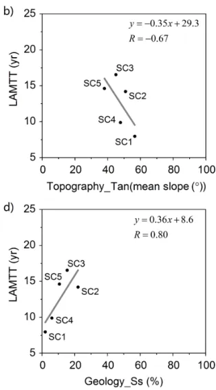
Soulsby et al. (2006b) showed a positive correlation between MTT and mean slope within the catchment,
354
while McGuire et al. (2005) found a negative correlation of MTT versus median flowpath gradient. In the
355
present study, MTT is inversely correlated with mean slope (Fig. 7b); however, the correlation coefficient is
356
smaller than that for some other factors.
357
Many previous studies (Soulsby et al., 2006a, b; Tetzlaff et al., 2009; Hrachowitz et al., 2010) have
358
highlighted that MTT decreases with increasing areal percentage of responsive soil cover (i.e., regosols,
359
peats, and gleys) within a catchment. However, in the present study, the correlation of MTT is not significant
360
with the coverage of any specific soil. Conversely, the areal percentage of forest and Ss show strong
361
correlation with MTT (Fig. 7c and d), whereas previous studies have never emphasized relationships
362
between MTT and specific land use/cover or geology.
363
The highest correlation was found between MTT and the storage amount of Layer 4 (Fig. 7e). Although
364
the lumped hydrologic model used in this study is a semi-conceptual one, Layer 4 implicitly corresponds to
365
groundwater storage. Soulsby et al. (2006b) clarified that MTT increases with increasing groundwater
366
contribution to a stream and our results are consistent with their finding.
367
As mentioned above, the factors likely to control MTT are storage of Layer 4, forest coverage, Ss
368
coverage, and mean slope; however, some factors correlate with each other (Table 4). To clarify the
369
independent (i.e., true) controlling factor(s), multiple linear regression (MLR) with a stepwise selection of
370
explanatory variables was applied. The first and second best MLR models were as follows:
371
372
MTT=0.358SL4+0.189CSs+4.613 (Adjusted-R2 = 0.988) (19)
373
MTT
=
0.471
S
L4
+
4.866
(Adjusted-R2
= 0.828) (20)
19 / 42 375
where SL4 (m) is the storage of Layer 4 and CSs (m2/m2) is the Ss coverage. This result suggests that the most
376
important factor controlling LAMTT is the storage of Layer 4, i.e., groundwater storage. In mountainous
377
areas, where mean slope is high and the dominant land use/cover is forest, good aquifers are thin and thus,
378
groundwater storage is expected to be small. Conversely, in the plains, groundwater storage seems to be
379
greater because of the thicker aquifers compared with mountainous areas. Large groundwater storage helps
380
water to age, which increases transit times.
381
The Ss coverage, which is the second important variable in the MLR models, is much higher in SC2 than
382
in the other SCs. In SC2, some tributaries of the Fuji River have formed alluvial fans with very thick
383
sediments, which are mainly composed of highly permeable sand–shale conglomerate. In such a catchment,
384
deep flowpaths through the thick sediments are expected to contribute considerably to river runoff. Indeed,
385
as for the model, the value of kV of Layer 4 in SC2 is the largest among all the SCs, strengthening deep
386
flowpaths. This indicates that groundwater contributions to river runoff in SC2 are represented not only by
387
Layer 4, but also by Layer 5. In other words, groundwater flow patterns in alluvial-fan-dominated
388
catchments seem to differ from those in other catchments. This is the reason why Ss coverage is the second
389
important factor, independent of the storage of Layer 4.
390
In short, groundwater storage is undoubtedly important as a factor controlling inter-catchment variation of
391
LAMTT. As shown in the previous section, inter-catchment variation of LAMTT reflects the difference of
392
MTT in dry periods more strongly. Although inter-catchment variation in wet periods could be affected by
393
other factors, such effects should be minor because the spatial variance of MTT in wet periods is small.
394
In previous studies, the importance of both groundwater storage and its topographic control has not been
20 / 42
emphasized. This is probably because small headwater catchments dominated by mountainous topography
396
have been the principal focus of study and few mesoscale catchments that include plains with large
397
groundwater storage have been investigated. In this context, the most dominant factor controlling the spatial
398
variation of MTT might be scale-dependent, even though catchment size is not a direct controlling factor.
399
400
5. Summary and conclusions 401
402
Time-variant MTTs of five SCs of the Fuji River catchment were estimated using a five-layer tank model,
403
calibrated and validated using observed river discharge and river water stable isotopes (i.e., δ18O and δD).
404
The monthly average MTTs ranged from several years to decades; the variation range and long-term
405
averages were different for all the SCs. However, the patterns of temporal variation of the estimated MTTs
406
were similar in all SCs. Inter-catchment variation of MTT was greater in dry periods than in wet periods.
407
The long-term average MTT in each SC was correlated with mean slope, coverage of forest (or conversely,
408
other land use types), coverage of sand–shale conglomerate, and groundwater storage. The use of multiple
409
linear regression revealed that inter-catchment variation of MTT is principally controlled by the amount of
410
groundwater storage, which is smaller in mountainous areas covered mostly by forests than in plain areas
411
with less forest coverage and smaller slopes. Such topographic control of MTT through the factor of
412
groundwater storage seems important in mesoscale catchments that include both mountains and plains.
413
To a greater or lesser extent, model-based estimates of MTT depend on the structure and/or accuracy of
414
the model. River discharge and river water isotopic compositions were well reproduced by the model, not
415
only in calibration periods, but also in the validation periods. Furthermore, the fact that inter-catchment
21 / 42
variation of MTT could be reasonably explained by catchment characteristics (e.g., topography, land use,
417
and geology) and internal parameters of the model (e.g., storage of Layer 4) supports the usefulness of our
418
approach. As the MTT is more strongly controlled by water storage than by flow, isotopic tracers sensitive to
419
water storage are shown to be important tools for calibrating/validating the model.
420
421
Acknowledgments 422
423
This study was supported in part by the Research and Education Funding for Japanese Alps
424
Inter-Universities Cooperative Project, Ministry of Education, Culture, Sports, Science and Technology,
425
Japan, and Japan Society for the Promotion of Science (JSPS) KAKENHI Grant Number 25·3813. The
426
authors would like to acknowledge Professor Jeff McDonnell for his invaluable suggestions. Comments
427
from the two anonymous reviewers were helpful in improving our manuscript.
428
429
References 430
431
Allen, R.G., Pereira, L.S., Raes, D. and Smith, M., 1998. Crop evapotranspiration: guidelines for computing
432
crop requirements, FAO Irrigation and Drainage Paper No. 56, FAO, Rome, Italy.
433
Blöschl, G., 2005. On the Fundamentals of Hydrological sciences, Encyclopedia of Hydrological Sciences.
434
3471, 3–12.
435
Bolin, B., Rodhe, H., 1973. A note on the concepts of age distribution and transit time in natural reservoirs,
436
Tellus. 25, 58–62.
22 / 42
Cappa, C.D., Hendricks, H.B., Depaolo, D.J., Cohen, R.C., 2003. Isotopic fractionation of water during
438
evaporation. J. Geophys. Res.108, D16–4525, doi:10.1029/2003JD003597.
439
Craig, H., Gordon, L.I., 1965. Deuterium and oxygen 18 variations in the ocean and marine atmosphere. In
440
proc. Stable Isotopes in Oceanographic Studies and Paleotemperatures, Tongiogi, E. (Eds.), pp. 9–130,
441
V. Lishi e F., Pisa, Spoleto, Italy..
442
DeWalle, D.R., Edwards, P.J., Swistock, B.R., Aravena, R., Drimmie, R.J., 1997. Seasonal isotope
443
hydrology of three Appalachian forest catchments, Hydrol. Process. 11(15), 1895–1906.
444
Druhan, JL., Maher, K., 2014. A model linking stable isotope fractionation to water flux and transit times in
445
heterogeneous porous media. Procedia Earth and Planetary Science 10, 179–188,
446
doi:10.1016/j.proeps.2014.08.054.
447
Duffy, C.J., 2010. Dynamical modeling of concentration–age–discharge in watersheds, Hydrol. Process. 24,
448
1711–1718.
449
Fovet, O., L. Ruiz, L., Faucheux, M., Molénat, J., Sekhar, M., Vertès, F., Aquilina, L., Gascuel-Odoux, C.,
450
and Durand, P., 2014. Using long time series of agricultural-derived nitrates for estimating catchment
451
transit times, J. Hydrol.522(2015), 603–617, doi:10.1016/j.jhydrol.2015.01.030.
452
Gat, J.R., Shemesh, A., Tziperman, E., Hecht, A., Georgopoulos, D., Basturk, O., 1996. The stable isotope
453
composition of waters of the eastern Mediterranean Sea. J. Geophys. Res. 101(C3), 6441–6452,
454
doi:10.1029/95JC02829.
455
Goode, D.J., 1996. Direct simulation of groundwater age. Water Resour. Res. 32(2), 289–296.
456
Hrachowitz, M., Soulsby, C., Tetzlaff, D., Speed, M., 2010. Catchment transit times and landscape controls–
457
does scale matter? Hydrol. Process. 24(1), 117–125.
458
Hrachowitz, M., Fovet, O., Ruiz, L., and Savenije, H. H. G., 2015. Transit time distributions, legacy
23 / 42
contamination and variability in biogeochemical 1/fα scaling: how are hydrological response dynamics
460
linked to water quality at the catchment scale?. Hydrol. Process., doi: 10.1002/hyp.10546.
461
Khatiwala, S., Visbeck, M., Schlosser, P., 2001. Age tracers in an ocean GCM, Deep-Sea Res.Pt. 48, 1423–
462
1441.
463
Kim, S. and Jung, S., 2014, Estimation of mean water transit time on a steep hillslope in South Korea using
464
soil moisture measurements and deuterium excess. Hydrol. Process., 28,1844–1857, doi:
465
10.1002/hyp.9722.
466
Klaus, J., Chun, K., McGuire, K., McDonnell, J.J., 2015. Temporal dynamics of catchment transit times
467
from stable isotope data. Water Resources Research, 51, 4208–4223, doi:10.1002/ 2014WR016247.
468
Kubota, T., Tsuboyama, Y., 2004. Estimation of evaporation rate from the forest floor using oxygen-18 and
469
deuterium compositions of throughfall and stream water during a non-storm runoff period, Journal of
470
Forest Research. 9, 51–59.
471
Love, D., Uhlenbrook, S., Zaag, P., 2011. Regionalising a meso-catchment scale conceptual model for river
472
basin management in the semi-arid environment, Physics and Chemistry of the Earth. 36, 747–760.
473
doi:10.1016/j.pce.2011.07.005.
474
Ma, W., Yamanaka, T., 2013. Temporal variability of mean transit time and transit time distribution assessed
475
by a tracer-aided tank model for a meso-scale catchment, Hydrological Research Letters. 7(4), 104–
476
109, doi: 10.3178/hrl.7.104.
477
Makino, Y. (2013), Mapping of Stable Isotopes in Precipitation over the Japanese Alps Region and Its Use
478
for Diagnosing Hydrological Cycle for Catchment Area, M.S. thesis, 81 pp., Univ. of Tskuba. at
479
Tsukuba, Japan, 28 February.
480
Majoube, M., 1971. Fraction0nement en oxygene-18 entre la glace et la vapeur d'eau. J. Chim. Phys. 68,
24 / 42
625–636.
482
Makihara, Y., 1996. A method for improving radar estimates of precipitation by comparing data from radars
483
and raingauges. J. Meteor. Soc. Japan. 74, 459–480.
484
Maloszewski, P., Zuber, A., 1982. Determining the turnover time of groundwater systems with the aid of
485
environmental tracers, I-Models and their applicability. J. Hydrol.57, 3–4. 207–231.
486
Maloszewski, P., Rauert, W., Stichler, W., Herrmann, A., 1983. Application of flow models in an alpine
487
catchment area using tritium and deuterium data. J. Hydrol.66, 319–330.
488
McDonnell, J.J., McGuire, K., Aggarwal, P., Beven, K.J., Biondi, D., Destouni, G., Dunn, S., James, A.,
489
Kirchner, J., Kraft, P., Lyon, S., Maloszewski, P., Newman, B., Pfister, L., Rinaldo, A., Rodhe, A.,
490
Sayama, T., Seibert, J., Solomon, K., Soulsby, C., Stewart, M., Tetzlaff, D., Tobin, C., Troch, P., Weiler,
491
M., Western, A., W¨orman, A., Wrede, S., 2010. How old is stream water? Open questions in
492
catchment transit time conceptualization, modeling and analysis. Hydrol. Process. 24, 1745–1754.
493
McGuire, K.J., DeWalle, D.R., Gburek, W.J., 2002. Evaluation of mean residence time in subsurface waters
494
using oxygen-18 fluctuations during drought conditions in the mid-Appalachians. J. Hydrol.261(1–4),
495
132–149.
496
McGuire, K.J., McDonnell, J.J., Weiler, M., Kendall, C., Welker, J.M., McGlynn, B.L., Seibert, J., 2005. The
497
role of topography on catchment-scale water residence time. Water Resour. Res. 41(5), W05002,
498
doi:10.1029/2004WR00365.
499
McGuire, K.J., McDonnell, J.J., 2006. A review and evaluation of catchment transit time modeling. J.
500
Hydrol. 330(3-4), 543–563.
501
Moriasi, D.N., Arnold, J.G., Van Liew, M.W., Bingner, R.L., Harmel, R.D., Veith, T.L., 2007. Model
502
Evaluation Guidelines for Systematic Quantification of Accuracy in Watershed Simulations,
25 / 42
Transactions of the ASABE. 50(3), 885–900.
504
Muñoz-Villers, L., Geissert, D., Holwerda, F., and McDonnell, J. J., 2015. Stream water transit times in
505
tropical montane watersheds: catchment scale and landscape influences. Hydrol. Earth Syst. Sci.
506
Discuss., 12, 10975–11011, doi:10.5194/hessd-12-10975-2015.
507
Nash, J.E., Sutcliffe, J.V., 1970. River flow forecasting through conceptual models part I-A discussion of
508
principles, J. Hydrol. 10(3), 282–290.
509
Ozyurt, N.N., Bayari, C.S., 2003. LUMPED: a Visual Basic code of lumped-parameter models for mean
510
residence time analyses of groundwater systems, Computers & Geosciences. 29, 79–90,
511
doi:10.1016/S0098-3004(02)00075-4.
512
Peters, NE., Burns, DA., Aulenbach, BT., 2014. Evaluation of High-Frequency Mean Streamwater
513
Transit-Time Estimates Using Groundwater Age and Dissolved Silica Concentrations in a Small
514
Forested Watershed. Aquat Geochem. 20, 183–202, doi:10.1007/s10498-013-9207-6.
515
Sayama, T., McDonnell, J.J., 2009. A new time-space accounting scheme to predict stream water residence
516
time and hydrograph source components at the watershed scale, Water Resour. Res. 45, W07401,
517
doi:10.1029/2008WR007549.
518
Scherrer, S., Naef, F., 2003. A decision scheme to indicate dominant hydrological flow processes on
519
temperate grassland. Hydrol. Process. 17(2), 39–401.
520
Seeger, S., Weiler, M., 2004. Reevaluation of transit time distributions, mean transit times and their relation
521
to catchment topography, Hydrol. Earth Syst. Sci., 18, 4751-4771, doi:10.5194/hess-18-4751-2014,
522
2014.
523
Shimada, J., Itadera, K., Nakai, N., Suprapta, DN., Gara, W., 1992. Stable isotope ratio in precipitation as an
524
input of hydrological cycle. In Water Cycle and Water Use in Bali Island, Kayane I (ed.). University of
26 / 42
Tsukuba: Tsukuba; 105–115.
526
Soulsby, C., Tetzlaff, D., Dunn, S.M., Waldron, S., 2006a. Scaling up and out in runoff process
527
understanding-Insights from nested experimental catchment studies, Hydrol. Process. 20, 2461–2465,
528
doi:10.1002/hyp.6338. 2006.
529
Soulsby, C., Tetzlaff, D., Rodgers, P., Dunn, S., Waldron, S., 2006b. Runoff processes, stream water
530
residence times and controlling landscape characteristics in a mesoscale catchment: an initial
531
evaluation. J. Hydrol. 325, 197-221.
532
Stockinger, M. P., Bogena, H. R., Lücke, A., Diekkrüger, B., Weiler, M., and Vereecken, H., 2014. Seasonal
533
soil moisture patterns: Controlling transit time distributions in a forested headwater catchment, Water
534
Resour. Res. 50, 5270–5289, doi:10.1002/ 2013WR014815.
535
Sugita, M., Tanaka, T., 2009. Hydrologic Science, Kyoritsu Shuppan Co, Japan, pp. 275.
536
Tetzlaff, D., Seibert, J., Soulsby, C., 2009. Inter-catchment comparison to assess the influence of topography
537
and soils on catchment transit times in a geomorphic province. Hydrol. Process. 23(13), 1847–1886.
538
Tetzlaff, D., Birkel, C., Dick, J., Geris, J., and Soulsby. C., 2014. Storage dynamics in hydropedological
539
units control hillslope connectivity, runoff generation, and the evolution of catchment transit time
540
distributions, Water Resour. Res., 50, 969–985, doi: 10.1002/2013WR014147.
541
Timbe, E., Windhorst, D., Celleri, R., Timbe, L., Crespo, P., Frede, H. G., Feyen, J., and Breuer, L., 2015.
542
Sampling frequency trade-offs in the assessment of mean transit times of tropical montane catchment
543
waters under semi-steady-state conditions, Hydrol. Earth Syst. Sci., 19, 1153–1168,
544
doi:10.5194/hess-19-1153-2015.
545
Uhlenbrook, S., Roser, S., Tilch, N., 2004. Hydrological process representation at the meso-scale: the
546
potential of a distributed, conceptual catchment model. J. Hydrol. 291, 278–296
27 / 42
Yamanaka, T., Shimada, J., Hamada, Y., Tanaka, T., Yang, Y., Wanjun, Z., and Chunsheng, H., 2004.
548
Hydrogen and oxygen isotopes in precipitation in a northern part of the North China Plain:
549
Climatology and inter-storm variability. Hydrol. Process. 18, 2211- 2222.
550
Yamanaka, T., 2009. Study on the atomspheric boundary layer using water vapor isotopes. K. Yoshimura, K.
551
Ichiyanagi and A. Sugimoto (Eds): "Use of Isotope Ratios of Water in Meteorology", Meteorological
552
Society of Japan, 61–76, Tokyo, Japan.
553
Yamanaka T., Onda Y., 2011. On measurement accuracy of liquid water isotope analyzer based on
554
wavelength-scanned cavity ring-down spectroscopy (WSCRDS). Bulletin of Terrestrial Environment
555
Research Center, University of Tsukuba,12, 31–40.
556
28 / 42 558
Figures: 559
560
Fig. 1. Map of study area and locations of isotopic monitoring sites and meteorological observation stations. 561
Here, Y1-Y5 represent isotopic collecting location. And, W1-W5 shows location of the Weather Station, 562
from where, meteorological observed data were collected, such as: temperature, precipitation, wind, solar 563
and others. ... 29
564
Fig. 2. Schematic illustration of five-layer tank model. ... 30
565
Fig. 3. Comparison between observed and simulated hydrographs. ... 31
566
Fig. 4. Comparison between observed and simulated isotope compositions. ... 32
567
Fig. 5. Comparison of MTT in monthly values among five SCs as well as monthly average precipitation for 568
the whole research area (i.e. SC5). ... 33
569
Fig. 6. Inter-catchment comparison of relationships between monthly average MTT and precipitation 570
amount for five SCs. ... 34
571
Fig. 7. Relationships of LAMTT with potential controlling factors in each SC. ... 35
572
573
574
575
576
577
29 / 42 579
Fig. 1. Map of study area and locations of isotopic monitoring sites and meteorological observation stations. Here, 580
Y1-Y5 represent isotopic collecting location. And, W1-W5 shows location of the Weather Station, from where, 581
meteorological observed data were collected, such as: temperature, precipitation, wind, solar and others. 582
30 / 42 584
Fig. 2. Schematic illustration of five-layer tank model. 585
586
31 / 42 588
Fig. 3. Comparison between observed and simulated hydrographs. 589
32 / 42 591
592
Fig. 4. Comparison between observed and simulated isotope compositions. 593
33 / 42 595
Fig. 5. Comparison of MTT in monthly values among five SCs as well as monthly average precipitation for the whole 596
research area (i.e. SC5). 597
34 / 42 608
Fig. 6. Inter-catchment comparison of relationships between monthly average MTT and precipitation amount for five 609
SCs. 610
35 / 42 613
Fig. 7. Relationships of LAMTT with potential controlling factors in each SC. 614
36 / 42 619
37 / 42 621
Tables: 622
Table 1. Characters of each catchment. ... 38 623
Table 2. Evaluation for simulations of (a) water balance and (b) isotope balance. ... 39 624
Table 3. Long-term statistics of estimated mean transit time on daily bases. ... 40 625
Table 4. Coefficients of correlation of LAMTT and potential controlling facotrs in each SC. ... 41 626
Table 5. Correlation matrix among potential factors controlling MTT. ... 42 627
628
629
630
631
38 / 42
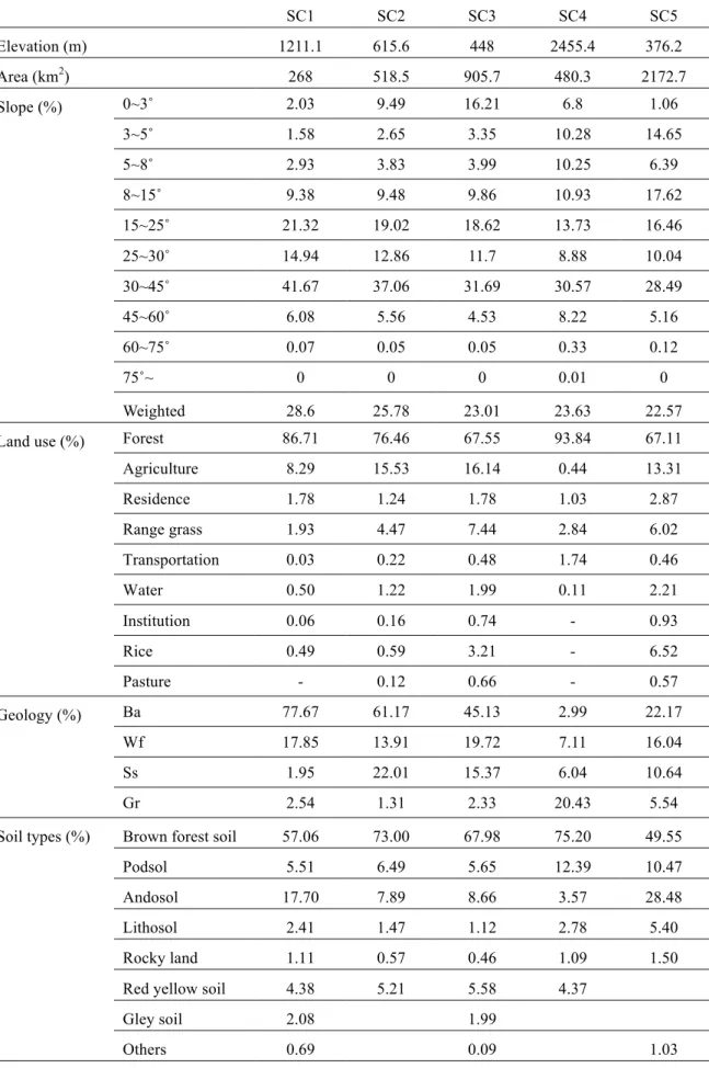
Table 1. Characters of each catchment. 633
SC1 SC2 SC3 SC4 SC5
Elevation (m) 1211.1 615.6 448 2455.4 376.2
Area (km2) 268 518.5 905.7 480.3 2172.7
Slope (%) 0~3˚ 2.03 9.49 16.21 6.8 1.06
3~5˚ 1.58 2.65 3.35 10.28 14.65
5~8˚ 2.93 3.83 3.99 10.25 6.39
8~15˚ 9.38 9.48 9.86 10.93 17.62
15~25˚ 21.32 19.02 18.62 13.73 16.46
25~30˚ 14.94 12.86 11.7 8.88 10.04
30~45˚ 41.67 37.06 31.69 30.57 28.49
45~60˚ 6.08 5.56 4.53 8.22 5.16
60~75˚ 0.07 0.05 0.05 0.33 0.12
75˚~ 0 0 0 0.01 0
Weighted 28.6 25.78 23.01 23.63 22.57
Land use (%) Forest 86.71 76.46 67.55 93.84 67.11
Agriculture 8.29 15.53 16.14 0.44 13.31
Residence 1.78 1.24 1.78 1.03 2.87
Range grass 1.93 4.47 7.44 2.84 6.02
Transportation 0.03 0.22 0.48 1.74 0.46
Water 0.50 1.22 1.99 0.11 2.21
Institution 0.06 0.16 0.74 - 0.93
Rice 0.49 0.59 3.21 - 6.52
Pasture - 0.12 0.66 - 0.57
Geology (%) Ba 77.67 61.17 45.13 2.99 22.17
Wf 17.85 13.91 19.72 7.11 16.04
Ss 1.95 22.01 15.37 6.04 10.64
Gr 2.54 1.31 2.33 20.43 5.54
Soil types (%) Brown forest soil 57.06 73.00 67.98 75.20 49.55
Podsol 5.51 6.49 5.65 12.39 10.47
Andosol 17.70 7.89 8.66 3.57 28.48
Lithosol 2.41 1.47 1.12 2.78 5.40
Rocky land 1.11 0.57 0.46 1.09 1.50
Red yellow soil 4.38 5.21 5.58 4.37
Gley soil 2.08 1.99