Labelling Method by Pupillometry forClassifying Attention Level by EEG/ECG/NIRS

(1)

九州大学学術情報リポジトリ

Kyushu University Institutional Repository

Labelling Method by Pupillometry for

Classifying Attention Level by EEG/ECG/NIRS

ゼニファ, ファディラ

https://doi.org/10.15017/4060012

出版情報：九州大学, 2019, 博士（システム生命科学）, 課程博士バージョン：

権利関係：

(2)

Labelling Method by Pupillometry for Classifying Attention Level by EEG-ECG-NIRS

Fadilla Zennifa

Graduate School of Systems Life Sciences Kyushu University

2020

(3)

2

Abstract

There are numerous methods to evaluate attention levels such as observation, self- assessment, and objective performance. This study aims to propose a new labeling method for attention levels detection by using parameter settings of pupillometry. This parameter setting then would be applied as data labeling in supervised machine learning toward EEG- ECG-NIRS.

To develop parameter settings of attention level evaluation, this study investigated the reaction of blink rates and pupillometry toward attention level based on self-assessment during cognitive tasks. My result showed there is no significant differences (P>0.05) in blink rates toward attention level within 10 seconds. On the other hand, pupillometry in low attention showed significant differences in pupillometry in the last 4 seconds cognitive tasks (P<0.05). After that, I calculated the distribution fit of pupillometry reaction in the attention level of all participants and plot the critical point of pupillometry data in 10 seconds and 4 seconds. After doing several experimental procedures, I chose parameter setting with a percentage of error of less than 15% and a different error 35 % compare with self assesment as future labeling method. Parameter setting which has been selected is when z-score within a specific range (-0.965 ≤ pupil ≤ 1.014) as high attention, other that range, will be classified as low attention.

Furthermore, I applied my labeling method for another physiological signal such as electroencephalograph (EEG), electrocardiograph (ECG), and near-infrared spectroscopy (NIRS). Numerous methods using electroencephalograph (EEG), electrocardiograph (ECG), and near-infrared spectroscopy (NIRS) for attention level detection have been proposed.

(4)

3 However, the results were either unsatisfactory or required many channels. In this study, I introduce the implementation of an EEG-ECG-NIRS for attention level detection. I used two- electrode wireless EEG, a wireless ECG, and two wireless channels NIRS to detect attention level during backward digit span, forward digit span and arithmetic. High attention will be labelled to data which has pupillometry z-score within specific range (-0.965 ≤ pupil ≤ 1.014) and another that range, will be classified as low attention. By using CFS+kNN algorithm, my result showed the accuracy system of EEG-ECG-NIRS (83.33± 5.95%) has the highest accuracy compare with EEG (81.90± 4.69%), ECG (82.51±3.57%), NIRS (78.37±7.12%).

Algorithm CFS+kNN also shown highest performance compare with other methods such as CFS+SVM (55.49± 27.89%), kNN (80.84± 3.88%) and SVM (55.88± 13.14%)

In summary, in this study, I established new parameter settings for evaluating attention level by using pupillometry and apply the parameter settings into EEG-ECG-NIRS to evaluate the EEG-ECG-NIRS performance, comparing with standalone system.

Keywords: labeling, supervised machine learning, blink rates, pupillometry, electroencephalograph, electrocardiograph, near-infrared spectroscopy, attention level detection

(5)

4

Ethics statement

The protocols for the present study were designed in accordance with the Declaration of Helshinki and were approved by faculty of information science and electrical engineering, Kyushu University (H26–3). Informed consent was obtained in writing from each participant

(6)

5

Chapter 1. General Introduction

Attention can be defined as the processing or selection of information at the expense of other information (Phashler et al., 1998; Anderson et al., 2004; Fougnie. 2008). Similarly, in 1890 psychologists and philosophers William James defines attention as taking possession by the mind, in clear and vivid form, of one out of what may seem several simultaneously possible objects or trains of thought. This implies withdrawal from some things to deal effectively with others (James. 1890). Attention also has been a key cognitive mechanism of interest in terms of differentiating among the various measures of time (Campbell et al., 2015). Knowing the human attention level helps improve human working and study efficiency (Berka et al., 2007; Sun et al., 2014). A study about attention in the psychology field was introduced by Wilhelm Wundt (Titchener., 1921). In 1868, Franciscus Donders investigated reaction time toward attention by using chronometry. Which the meaning of chronometry is the study about temporal sequencing of information in the brain (Donders.

1969). In the 1990s, positron emission tomography (PET) is started to be used for attention studies (Petersen et al., 1988; Posner and Petersen. 1990; Burton et al., 1999). In 1993, Osman et al (Osman et al., 1993) mentioned that attention can also affect EEG signals associated with later central processing stages, such as those involved in the selection and initiation of responses. Research about attention also has been investigated by using Electrocardiogram (ECG) (Borger et al., 1999; Smallwood et al., 2004; Griffiths et al., 2017).

Investigation of attention toward hemodynamic activity has been measured by using Near- Infrared Spectroscopy (NIRS) (Matsuda and Hiraki. 2006; Toichi et al., 2004; Derosière et al., 2013). Nowadays researchers are not only trying to investigate the effect of attention

(9)

8 toward physiological activity, but also trying to establish some methods to detect attention level automatically.

Generally, there are two main tasks in machine learning. They are unsupervised and supervised machine learning (Russel et al., 2010). The main differences between the two types are that supervised learning is done by data labeling and the goal is to learn a function that given a sample of data and desired output. Supervised machine learning is a method in machine learning by using knowing labeling methods to label the data and has the expecting result (input-output pairs) (Stuart et al., 2010). Unsupervised machine learning, on the other hand, is not based on data labeling and its goal is to infer the natural structure present within a set of data points. Measuring human mental states based on physiological activity has also been investigated by integrating EEG and ECG features (Stikic et al., 2014). The unsupervised method has been applied for cognitive state recognition in that experiment.

However, the unsupervised learning requires large amounts of data to get an appropriate pattern and also there is no certain validation method to validate the data. In my study, data labeling relied on physiological activities.

Inattention level detection, there are 4 methods commonly used. They are observation, objective performance, self-assessment, and physiological activity. The classification of attention based on self-reporting and observation tends to be delayed, sporadic, and intrusive.

Performance-based information can be misleading since multiple degrees of tasks could be grouped with the same level of performance. Conversely, physiological measures can be arranged to have little or no interference with task execution and can supply information

(10)

9 continuously without significant delay (Yurko et al., 2010; Sun et al., 2014; Aghajani et al., 2017).

This study aims to label attention level using pupillometry, which can be further used in a supervised machine learning system of attentional evaluation. In this thesis I focused on how to establish the algorithm for new labeling by using pupillometry, after that, I applied the label and established the model algorithm based on supervised machine learning on EEG- ECG-NIRS for attention level detection.

As the task design, I used common attention task test which is digited span forward and backward (Jensen et al., 1975; Cullum., 1998; Berka et al 2007, Zennifa et al., 2018; Zennifa et al., 2019), and additionally, I also applied the arithmetic test (Zennifa et al., 2018; Zennifa et al., 2019). Most of the questions in this experiment were relatively simple and did not require any prerequisite knowledge or specific skills. However, a good level of attention and alertness was required to avoid making easy mistakes. There were several problems need to solve before taking the experiment. All participants had a normal visual function, were not with a disability and could do the experiment without wearing glasses. I also asked participants to have breakfast and not drink any caffeine before taking the test. Some participants did not follow this rule, and we have to exclude their data.

I am currently implementing a parameter setting based on features of pupillometry and for data labeling, I used Weka 3.8 (Hall et al., 2009) data mining for machine learning. I also applied a CFS + KNN algorithm on an EEG-ECG-NIRS system and used a searching algorithm which is called “best first”.

(11)

10 In the next section, I reviewed basic knowledge of attention level detection and blink rates, pupillometry and also EEG-ECG-NIRS. Furthermore, I introduced the related literature about attention level detection.

1.1 Some basic notions 1.1.1 Attention level detection.

Attention is the behavioral and cognitive process of selectively concentrating on a discrete aspect of information, whether deemed subjective or objective while ignoring other perceivable information. Knowing human attention is useful for efficiency in both working and studying (Berka et al., 2007, Sun et al., 2014).

There are 178 journals and magazines about attention level detection in the current past 10 years based on IEEE explore. There are 16 articles about “attention level detection” based on google scholars within 10 years. There are 139 journal articles about “attention pupillometry” based on pubmed.gov. Attention level detection has been done (by D.Das et al., 2013) in two classifications high attention and low attention based on behavioral pattern analysis. They used a robot as an observer to captures the attention of the person. But this research purely based on participant behavior. Another researcher (Sun et al., 2014), by using facial expression try to detect the attention level which accuracy up to 77.81%. By using facial expression is also depends on country culture. (Hussain et al., 2014) investigated the activity of physiological signals and facial responses to cognitive load under an emotional stimulus and collected participant ratings from a self-assessment manikin to find the normative ratings in the collection. They investigated the correlation between physiological data and the level of stimulation. They also subsequently compared the accuracy of cognitive

(12)

11 load detection with face video features, physiological features, and participant rating features with fusion features. They concluded that classification with fusion features (i.e., not only based on self-report) performed with more accuracy. In my study, I proposed to establish a new labeling method for attention level detection and using the labeling data to train data from EEG-ECG-NIRS.

1.1.2 Blink rates and Pupillometry

In this study, I used EOG (electrooculogram) to measure blink rates and eye tracker to record pupillometry. EOG records eye movements by measuring electrical potential differences between two electrodes. This takes advantage of the fact that the human eye is an electrical dipole consisting of a positively charged cornea and a negatively charged retina, first discovered by Schott in 1922 (Muller et al 2016). When I used EOG, blink specify by amplitude more than 150 μV (Zennifa et al 2018.,; Bulling et al., 2011; Abo-zahhad et al., 2015; He S., 2017). Blink rates are the number of blinks at specific times. Eyeblinks are actively involved in the release of attention (Nakano et al, 2013). (Marc et al, 2015) evaluated spontaneous eye blink rate (SEBR) and percentage of incomplete blinks in different hard- copy and visual display terminal (VDT) reading conditions, compared with baseline conditions. In that study, they concluded that high cognitive demands associated with a reading task led to a reduction in SEBR, irrespective of the type of reading platform. However, only electronic reading resulted in an increase in the percentage of incomplete blinks, which may account for the symptoms experienced by VDT users. Blinking has been correlated with cognitive activity (Paprocki et al., 2017). Their study mentioned that blink rate carry information about cognitive performance and can be employed in the assessment of cognitive

(13)

12 abilities without taking a test. Blink rate for mental states is performed by (Ren et al., 2019) in their paper, they attempted to differentiate between high and low cognitive loads of an individual through the analyses of BR and BRV (blink rate variability). The result indicated that BRV achieves significantly higher AUC values than BR, which suggests its strong potentiality for MSR. In sum, the BRV may prove to be a promising method for the MSR, which should be considered in the future.

Pupillometry is the measurement of pupil size and reactivity. It is also used in psychology (Granholm et al., 2004). Pupillometry is concerned with changes in pupil size. The diameter of the pupil size has long been known as a marker of cognitive load and attentional performance (Karatekin et al., 2007; Tsukahara et al., 2016; Hartmann et al, 2014; Geva et al., 2013; Unsworth et al., 2017 a&b; Piquado et al., 2010). A study by (Rud L van Den et al., 2016) mentioned that pupil size could be used to track the focus of attention. (Smallwood et al., 2011) concluded in their research that pupil dilations not only provide an index of overall attentional effort but are time-locked to stimulus changes during attention (but not during mind-wandering). This finding suggests that pupil dilations afford a dynamic readout of conscious information processing. Their finding later has been duplicated buy (Kang et al., 2014), demonstrating stimulus-pupil coupling from reflects online cognitive processing beyond sensory gain. The usage of pupillometry for attention research also used by (Naber et al., 2013). In their research, they used pupil frequency tagging (PFT) method to see the connection between cortical centers with visual selective attention. They concluded that the amplitude of pupil responses closely follows the allocation of focal visual attention and the encoding of stimuli. (Van der Wel et al., 2018).

(14)

13 1.1.3 EEG, ECG, NIRS research toward attention

Numerous methods using electroencephalograph (EEG), electrocardiograph (ECG), and near-infrared spectroscopy (NIRS) for the recognition of attention level and cognitive tasks have been proposed (Iramina et al., 2010; Zennifa et al.,2015; Shin et al., 2018; )). A study by (Chang et al., 2012) examines the brain oscillatory activities and peripheral physiological measures were influenced by attention levels. In their study, the level of attention is based on task difficulty. Their research mentioned that heart rate, heart rate variability, response rate, eye blinks, and skin conductance could be considered as promising indices for discriminating attention levels.

A wearable integrated electroencephalograph (EEG) and electrocardiograph (ECG) has been adapted for measuring the change of neurophysiological and autonomic activity in attention level, for autism spectrum disorder children. Attention level, which is determined as engagement states are labeled by observation method from 2 observers. By extracting quantitative EEG (QEEG) features from an EEG signal, as well as heart rate and heart rate variability (HRV) from an ECG, they found evidence of differing activity in the engagement and disengagement states, in both the EEG and ECG (Billeci et al., 2016). Near-infrared spectroscopy (NIRS) has been applied to assess anterior frontal hemodynamic responses to attention during three cognitive tasks. In their study, instead of doing engagement detection, they presented evidence of age-related anterior frontal hemodynamic changes with cognitive demands. (Bierre et al., 2017). Another attention level detection has also done by using SSVEP (Punsawad et al., 2017), the attention is categorized based on the EEG signal when the alpha ratio is decreased, and the beta ratio is increased than baseline. They got the

(15)

14 accuracy of their data based on an algorithm is 81 %. (Liu et al., 2013) developed attention recognition by using single channels EEG. The labeling process in their research used participant self-assessment. In their research, they found the accuracy signal is 76.82% by using the SVM algorithm.

1.2 Thesis overview

This thesis consists of 4 chapters. Chapter 1 talking the general introduction of my study.

I mentioned several studies that have done a similar experiment or some studies which become the basis of this study.

Chapter 2, I explained about the effect of blink rates and pupillometry toward attention level. In this chapter, we compared several methods for attention level detection such as; self- assessment, objective performance, observation, and our quantitative formula. I also explained the process to develop an algorithm for labeling the data to our model (EEG-ECG- NIRS) this chapter is based on the study by (Zennifa et al., 2019). The experiment in this chapter has been done for investigating the blink rates and pupillometry and evaluate it based on participant self-assessment.

Chapter 3, I talked about the application of the quantitative formula in supervised machine learning to our model (EEG-ECG-NIRS). In this chapter, participants did BDS, FDS, arithmetic tasks. For each task, there were three different cognitive task levels: Level one consisted of 30 trials with four digits in each trial; Level two consisted of 30 trials with five digits in each trial, and level three consisted of 30 trials with six digits in each trial. I recorded EEG, ECG, NIRS, eye tracking and EOG simultaneously. These experiments aim to collect

(16)

15 the data and applied the quantitative formula in data labeling for further application in supervised machine learning.

Chapter 4, The last chapter in this study, we talked about the general discussion of this thesis. This chapter aims to mention all founding that we have and the limitation of my study.

1.3 Purpose of this study

I am currently implementing an EEG-ECG-NIRS (hybrid technology system) that can be used to evaluate attention levels during cognitive tasks. Several studies on the hybrid system have mentioned their promising characteristics. (Ahn et al., 2017) have suggested computational integration methods to achieve a hybrid EEG-NIRS system for mental fatigue states. However, the multimodal EEG-NIRS system in their study is a high-density type, which requires many channels data. (Hong et al., 2018) focused on the utility of the integration between EEG and NIRS for locked-in syndrome patients. They mentioned that the proper selection of features will improve the accuracy of classification. In my study, I investigated the features that can be used in attention level detection; the difference lies in the approach of the study. (Ahn et al., 2016) combined EEG, ECG, and NIRS by using 68 electrodes for EEG, ECG, and EOG and 8 channels in the NIRS in simulated driving. In my study, I use a two-electrode EEG, an ECG, and two channels in the NIRS. All the mentioned sensors are wireless. Previous work (Iramina et al., 2010; Zennifa et al., 2015) used this system for monitoring the cognitive state in children with developmental disorders during a 7 year training period. This time I would like to do attention level detection of the low-density hybrid system.

(17)

16 I investigated nine types of linear and nonlinear features from EEG, ECG, and NIRS to find the most common features that can be used in attention level detection. The investigation of linear and nonlinear features has been previously studied for mental state recognition but in stand-alone systems, such as only for EEG or ECG (Zakeri et al., 2017; Li et al., 2018; Huang et al., 2018). In my study, I tried to adapt these features to the hybrid system. This step was improved by combining the feature selector and classifier. I used the correlation-based feature selection (CFS) introduced by (Hall., 1999) as the feature selector and k-nearest neighbor (kNN) as the classifier, following several comparisons with other classifiers. Although a CFS and kNN combination (CFS + kNN) algorithm with two types searching method (i.e., best first search and greedy stepwise search) has been used by (Hu et al., 2018). My study applied a CFS + kNN algorithm in a low-density hybrid system and used one searching algorithm. In conclusion, the aim of this study is to propose a new labeling method for attention level recognition using pupillometry and applied it in EEG – ECG – NIRS system.

(18)

17

Chapter 2. New Labelling method for attention level detection

2.1 Abstract

Attention is described as a state in which an individual involved in an activity can ignore other influences. The attention level is important to obtain good performance, especially under study conditions. Numerous methods for attention level detection such as observation, self-assessment, objective performance and physiology signal has been applied. In this chapter, I tried to develop a labelling method based on physiological data (blink rates and pupillometry).

In this chapter, I compared the self-assessment method with other attention level detection methods (observation and objective performance). The aim of this comparison is to know the differences evaluation between self –assessments and other methods. From this comparison, I got the difference of self-assessment toward other method is lower than 21%.

After that, I investigated the effect of attention level based on self-assessment to blink rates, and pupillometry. I found that pupillometry in low attention is smaller than high attention especially in the last 4 second encoding time (P<0.05). On the other hand, I did not get a significant difference in blink rates. After that, I calculated the distribution fit of pupillometry reaction in the attention level of all participants and plot the critical point of pupillometry data in 10 seconds and 4 seconds. After doing several experimental procedures, I chose parameter setting by comparing with self-assessment with a percentage of error of less than 15% and a different error 35 % as future labeling method. Parameter setting which has been selected is when z-score within a specific range (-0.965 ≤ pupil ≤ 1.014) as high attention, other that range, will be classified as low attention.

(19)

18 2.2. Materials and Methods

2.2.1 Participants

There were 18 participants in my experiment. All participants were Kyushu University students, with ages ranging from 21 to 29 (23.5 ± 2.18). All participants had a normal visual function and were free of disability; 15 were right-handed, 1 participant was ambidextrous, and 2 participant was left-handed. Participants were instructed not to consume any caffeine 2 h before the experiment because it could affect the HRV (Martínez-Sellés et al., 2013;

Oliveira et al., 2017). The study was conducted by following the ethical principles of Kyushu University and the Declaration of Helsinki. Written informed consent was obtained from each participant before the experiment as showed on Appendix 1.

2.2.2 Experiment condition

The experiment took place in a dimly lit room. I also recorded the behavior activities using a webcam camera (Logicool C270, Logitech, Switzerland), which was located around 57 cm in front of the participant’s face.

Three types of attention task were used: backward digit span (BDS) (Jensen et al., 1975;

Cullum., 1998; Berka et al 2007, Zennifa et al., 2018; Zennifa et al., 2019; Rosenthal et al., 2006), forward digit span (FDS) (Jensen et al., 1975; Cullum., 1998; Berka et al 2007, Zennifa et al., 2018; Zennifa et al., 2019; Rosenthal et al., 2006) and arithmetic (Zennifa et al., 2018). These tasks consist of three-level. Level one consisted of a series of 20 sets of four digits, level two: 20 sets of five digits and level three: 20 sets of six digits. Most of the questions in this experiment were relatively simple and did not require any prerequisite knowledge or specific skills. However, a good level of attention and alertness was required

(20)

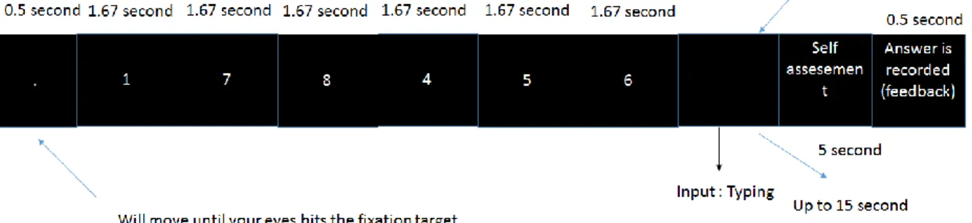
19 to avoid making easy mistakes because the response time was limited to 15 s. Each trial started with the presentation of a central, white fixation dot on a dark background until the participant’s eyes could be accepted by the eye tracker. Next, cognitive questions (i.e., encoding session) would appear for 10 s and the participant was instructed to respond within 15 s. Digits will appear every 2.5 seconds in 4 digit level, 2 seconds in 5 digit level and 1.67 seconds in 6 digit level. After that, participants should report their attention level in two conditions, high or low. All cognitive tasks were counterbalanced. The measurement was recorded after the practice session finished. The task can be seen in Figure1.

Figure 1. Task design example

2.2.3. Software and Apparatus

In this chapter, the 17-inch CRT monitor (1024 × 768) has been used for presenting the stimuli. Testing took place in a dimly lit room. Stimuli presentation was done by using OpenSesame (Mathôt et al., 2012), using the legacy back end for the display control and the PyGaze toolbox (Dalmaijer., 2014) for integrating to the eye tracker.

(21)

20 2.2.3.1 Eye Tracking

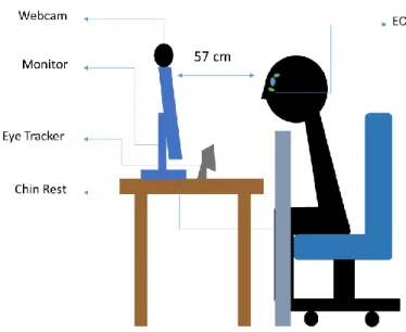
Before the start of each task, participants were positioned in front of an eye tracker (The EyeTribe tracker version 1, Copenhagen, Denmark). The distance of the participants' eyes from The EyeTribe was estimated to be ~57 cm. The participants were asked to fix their heads on a chin rest. In this study, we calibrated and validated the eye-tracking system to each participant using a nine-point dot matrix. After validation, the eye tracker that had been embedded with the OpenSesame software labeled each calibration point with the error in the degree of the visual angle between the calibrated and validated measures. If the calibration points do not exceed 1° (degree) and the greatest single point error does not exceed 1°, the process would continue. Before each trial, a one-point eye tracker recalibration was performed.

2.2.3.2 Electrooculogram

In this study, EOG (Polymate Mini AP 108, Miyuki Giken Co., Ltd., Kasugai-city, Japan) signals were sent by Bluetooth to a computer. The frequency of sampling was 500 Hz. We put two electrodes for a vertical EOG. This location was chosen to detect blink(Waters et al.,2005 ; Huang et al, .2018). Figure 2 shows the electrode placements.

(22)

21

Figure 2. Position of the participant during the experiment

2.3 Data Analysis

2.3.1 Comparison system from all attention level detection method

In this study, I compared the accuracy recognition from self-assessment to another detection method (observation and performance). This analysis aims to know the similarity accuracy recognition. The example of calculation can be seen in Table 1.

Table 1. Accuracy comparison self-assessment vs other methods.

Other parameters Self-assessment Status

High High True

Low High False

Low Low True

(23)

22 Based on data from Table 1, I calculated difference rate error and error rate detection based on formula (1) and formula (2).

Difference error is difference status between self-assessment and another method in each trial.

Error detection is the different status between self-assessment and another method in all trials.

Total trials means the number of all trials that has been done by each participant.

2.3.2 Blink rates and pupillometry analysis

After getting results from participant self-assessment and another recognition method, I started to analyze the blink rates and pupillometry. I would like to check the effect of attention based on self-assessment toward blink rates and pupillomery. Below is the explanation how do I analyze blink rates and pupillometry.

2.3.2.1 Blink rates

I used EOG to detect the blink rates of our participants every 10 seconds (encoding time).

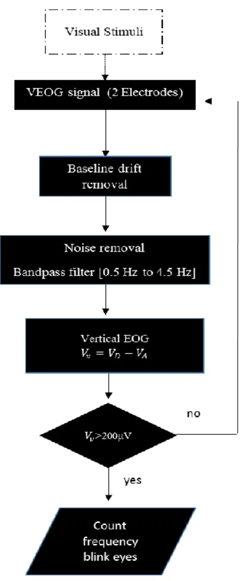
Blinking has been correlated with cognitive activity. In this study, eye blinks were detected with vertical EOG. To analyze the EOG signal, I used MATLAB 2017b. We performed baseline drift removal. The EOG signal is characterized by a frequency range of 0.1 to 20 Hz, and the amplitude lies between 25 and 3500 μV. We applied a bandpass filter from 0.1 to 20 Hz. I selected the detected peak at more than 200 μV as the criterion (Bulling et al., 2011) for eye blinking. The process of blink detection is explained in Figure 3, as follow:

difference rate detection (%) = 𝑑𝑖𝑓𝑓𝑒𝑟𝑒𝑛𝑐𝑒 𝑒𝑟𝑟𝑜𝑟 𝑡𝑜𝑡𝑎𝑙 𝑡𝑟𝑖𝑎𝑙𝑠 (1) error rate detection (%) =𝑒𝑟𝑟𝑜𝑟 𝑑𝑒𝑡𝑒𝑐𝑡𝑖𝑜𝑛

𝑡𝑜𝑡𝑎𝑙 𝑡𝑟𝑖𝑎𝑙𝑠 (2)

(24)

23

Figure 3. Blink detection

2.3.2.2 Pupillometry analysis

Pupillometry is concerned with changes in pupil size. The diameter of the pupil size has long been known as a marker of cognitive load and attentional performance. A study by (Van Den et al., 2016) mentioned that pupil size could be used to track the focus of attention.

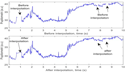
When using eye-tracking for recording pupil size, there was missing data. To solve the problem, I did cubic spline interpolation (Koening et al., 2017; Kang et al., 2014; Dalmeijer et al., 2014; Van der Brink et al 2014) in our data to reconstruct the signal, and connecting

(25)

24 the missing data. Figure 4 is shown signal differences before interpolation and after interpolation.

Figure 4. Signal reconstruction

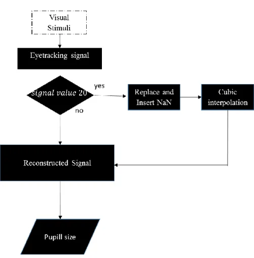
In this study, I analyzed pupillometry using a handmade program written in Matlab 2017b. The process is started by detecting missing data or signal with less than 20 pixels will be replaced with NaN then applied cubic interpolation to reconstruct the data.

The analysis process can be seen in Figure 5.

(26)

25

Figure 5. Pupillometry analysis

After getting the value of pupil size, considering difference of each individual data, I converted the value of raw pupillometry to Z-score, as showed in Equation (3):

Zpupil=𝑥𝑠𝑎𝑚𝑝𝑙𝑒−𝜇𝑝𝑜𝑝𝑢𝑙𝑎𝑡𝑖𝑜𝑛 𝑆𝑑_{𝑝𝑜𝑝𝑢𝑙𝑎𝑡𝑖𝑜𝑛} (3) Where 𝑥_{𝑠𝑎𝑚𝑝𝑙𝑒} is participant pupillometry in each trial.

𝜇_{𝑝𝑜𝑝𝑢𝑙𝑎𝑡𝑖𝑜𝑛} is average participant pupillometry in all trials.

𝑆𝑑_{𝑝𝑜𝑝𝑢𝑙𝑎𝑡𝑖𝑜𝑛}is standard deviation of pupillometry in all trials 2.3.2.3 Data balancing

Because my data based on states (High attention and Low attention) are imbalances, I need to anticipate this event by re-sampling my data (Chicco et al, 2017). In my study, I applied oversample technique as solution for my imbalance data. Oversampling means to increase the number of minority

(27)

26 class members in dataset. By using over-sampling there is no information from the original training set is lost since all members from the minority and majority classes are kept. (Rahman et al., 2013;

Chawla et al., 2018). Balancing is applied when plotted histogram all participants data into one dataset.

2.4 Results

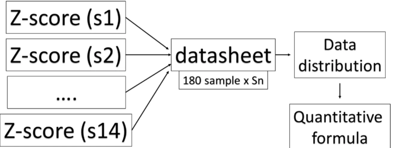
There are 18 participants joined to this experiment, but four of them has to be excluded due to technical problem. In this thesis, we used 14 participant’s data to establish the algorithm. Considering there was a difference in each participant’s physiological activity, we calculated the value of participants z-score based on Equation (3) to normalized the data and manage the data into one datasheet. There are data point 2520 in my datasheet. Data management can be seen in Figure 6.

Figure 6. Data management

(28)

27 2.4.1 Self-assessment reliability for the basis on quantitative formula

2.4.1.1 Self-assessment vs Objective behavior

This part, I tried to investigate the difference between self-assessment and objective behavior toward attention level detection. Based on objective behavior, if the participant’s response in a trial is incorrect, the current level of attention is marked as “low attention”; In contrast, if the response is correct, the current attention level is marked as “high attention.

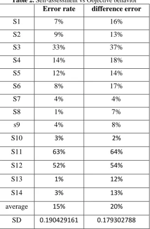
Based on formula (1) and (2) I compared the objective behavior and self-assessment. From this calculation, I found that the average error rate is 15±19.0 % and the average error is 20±17.9%. The detail can be seen in Table 2.

Table 2. Self-assessment vs Objective behavior Error rate difference error

S1 7% 16%

S2 9% 13%

S3 33% 37%

S4 14% 18%

S5 12% 14%

S6 8% 17%

S7 4% 4%

S8 1% 7%

s9 4% 8%

S10 3% 2%

S11 63% 64%

S12 52% 54%

S13 1% 12%

S14 3% 13%

average 15% 20%

SD 0.190429161 0.179302788

(29)

28 2.4.1.2 Self-assessment vs Observation

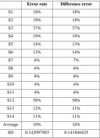
Similar to the previous part, in this part, we also investigated the difference between self- assessment and observation methods regarding attention level detection. Observation has been done by the author of this thesis and in this thesis, high attention is defined when the participant's eyes look at the monitor. When participants look away from the monitor, we categorized it as low attention. From our calculation we got the average error rate is 16±14.2%, difference error is 16±14.1%. The detail can be seen in Table 3.

Table 3. Self-assessment vs Observation

Error rate Difference error

S1 18% 18%

S2 18% 18%

S3 37% 37%

S4 19% 19%

S5 14% 13%

S6 13% 14%

S7 6% 7%

S8 6% 6%

S9 8% 8%

S10 4% 4%

S11 4% 4%

S12 58% 58%

S13 12% 11%

S14 11% 11%

Average 16% 16%

SD 0.142097983 0.141846425

2.4.1.3 Blink rates histogram based on self-assessment

I calculated blink rates of 14 participants during 180 trials. When I performed a t-test to compare the blink rates during that high attention and low attention, with alpha value 0.05,

(30)

29 By doing a t-test, I found there is no significant difference (P=0.605678). Blink rates data can be seen in Table 4.

Table 4. Blink rates during trials

High attention Low attention

S1 1 2

S2 1 0

S3 3 2

S4 1 1

S5 1 1

S6 1 2

S7 3 4

S8 3 4

S9 1 1

S10 1 1

S11 3 3

S12 3 3

S13 1 1

S14 5 6

Average 1.997974 2.066987

SD 1.339705 1.517106

2.4.1.4 Pupillometry based on self-assessment

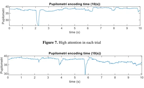
I calculated pupillometry based on temporal analysis and I divided the data based on self-assessment classification. Based on my investigation, I found pupillometry during high attention (Figure 7) and low attention (Figure 8) has a different characteristic.

(31)

30

Figure 7. High attention in each trial

Figure 8. Low attention in each trial

After calculating the data from each participant in each trial, I found that average pupil size in pupillometry has a tendency to be decreasing in low attention and tends to be stable in high attention in the temporal analysis. Following that, I also found that pupillometry in high attention has a bigger size rather than in low attention.

Figure 9. Temporal analysis pupillometry n= 14

(32)

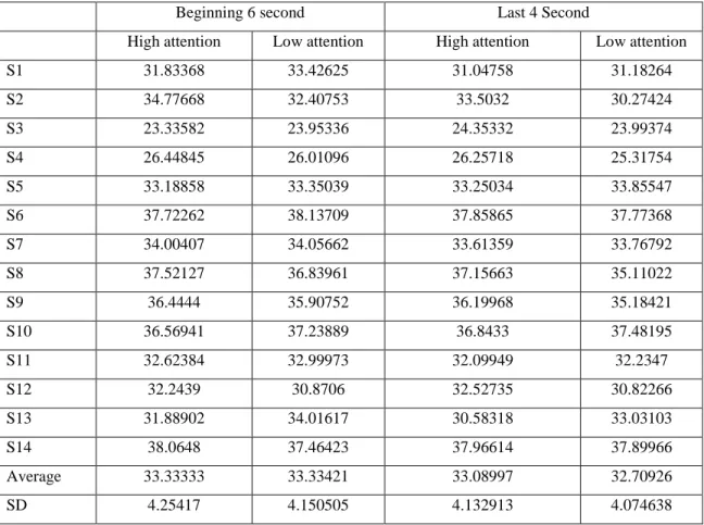
31 I did the further investigation by calculating the differences of pupillometry activity at the beginning of 6 seconds and the last 4 seconds of the encoding task from Figure 9 on this two attention levels. I found there is no significant difference (P>0.05) by using Wilcoxon rank-sum on the continues signal in beginning of 6 seconds. But I found there is significantly different on the continues signal by using Wilcoxon rank-sum test (P<0.05) last 4 seconds. Table 5 shows the average pupillometry in each participants based on attention levels.

Table 5. Average pupillometry in each subject

Beginning 6 second Last 4 Second

High attention Low attention High attention Low attention

S1 31.83368 33.42625 31.04758 31.18264

S2 34.77668 32.40753 33.5032 30.27424

S3 23.33582 23.95336 24.35332 23.99374

S4 26.44845 26.01096 26.25718 25.31754

S5 33.18858 33.35039 33.25034 33.85547

S6 37.72262 38.13709 37.85865 37.77368

S7 34.00407 34.05662 33.61359 33.76792

S8 37.52127 36.83961 37.15663 35.11022

S9 36.4444 35.90752 36.19968 35.18421

S10 36.56941 37.23889 36.8433 37.48195

S11 32.62384 32.99973 32.09949 32.2347

S12 32.2439 30.8706 32.52735 30.82266

S13 31.88902 34.01617 30.58318 33.03103

S14 38.0648 37.46423 37.96614 37.89966

Average 33.33333 33.33421 33.08997 32.70926

SD 4.25417 4.150505 4.132913 4.074638

I plotted data of all participants in all trials into one histogram. Plotting the data into one dataset and a histogram has been decided due to the small numbers of my data. So

(33)

32 instead plotting the histogram of 14 data point (because there are 14 participants), I plotted histogram of 14 participants in all trials, and it cause my data points become 2520. Those data can be seen on Figure 10. I plotted pupillometry histogram data into 3 areas. Two areas are considered a critical area and one area is considered as non-critical area. The critical area is defined as anything less than the standard deviation, the non-critical area is defined as anything that greater than the standard deviation. From this histogram, the most frequent value from all participants during high attention is 35.75 and the most frequent value of low attention is 32.91.

Figure 10. States last 4 second

Considering different activities from each participant, we converted raw pupillometry data into z- score value based on equation 4 and processed like Figure 6 in each participant and convert them into one data sheet and plot histogram. Based on Figure 11, the most frequent value in high attention is 0.475 and low attention most frequent value is 0.107.

(34)

33

Figure 11. Z-score last 4 second

2.4.2 Parameter settings for attention level

2.4.2.1 Extracting Pupillometry in 10 s to parameter settings

In this session, I tried to extracted data from histogram distribution during high attention and low attention to several thresholds for labeling. Average of ten-second data is used and converted to z-score, I divided data into 3 criteria (2 critical areas and 1 noncritical area). For further labeling is extracted from data in the non-critical area. The process to extract parameter setting for labeling is as follow:

(35)

34 The first parameter setting in this method has been taken on the most frequent value of pupil during low attention (-0.535) and the maximum value of pupil high during high attention. In this case, if z- score of pupil equal or more than 0.025 and lower or equal to 2.972 data will be labeled as low attention.

The second parameter setting is extracted from the most frequent value during high attention (0.5105). If z- score of pupil size is bigger than or equal to 0.5105 we labeled the data as high attention.

Parameter setting 1 If -0.535 < pupil So (“high attention”)

Else (“low attention”)

(36)

35 The third parameter setting is extracted from the mean value of pupillometry during high attention (0.938). High attention will be labeled to data which has a value bigger than 0.938

The fourth parameter setting is extracted from the minimum value of pupillometry during low attention (-1.07) and the maximum value of pupillometry during low attention (0.938).

Parameter setting 2 If 0.5105 ≤ pupil So (“high attention”)

Parameter setting 3 If 0.938 < pupil So (“high attention”)

(37)

36 The fifth parameter setting is based on a minimum value of pupillometry during high attention (-0.987) and minimum value during high attention (1.011). If z fulfilled the criteria, the data will be labeled as high attention.

The sixth parameter setting is based on the most frequent value of pupillometry during high attention (0.5105) and the maximum value of pupillometry (1.011). If the Z score of pupil size is fulfilled that criteria, data is labeled as high attention.

Parameter setting 4 If

-1.07 ≤ pupil ≤ 0.938 So (“low attention”)

Else (“high attention”)

-0.987 ≤ pupil ≤ 1.011 So (“high attention”)

(38)

37 The seventh parameter setting is based on the minimum value of pupillometry during low attention (0.5105). If the Z score of pupil size is fulfilled the criteria, we labeled the data as low attention.

The eight parameter setting is based on the mean value of pupillometry during high attention (0.012). If the Z score is fulfilled that criteria, we labeled the data as low attention.

0.5105 ≤ pupil ≤ 1.011 So (“high attention”)

Parameter setting 7 If pupil < 0.5105 So (“low attention”)

(39)

38 The ninth algorithm is based on a minimum value of pupillometry during low attention (-0.066). If the Z score of pupil size is lower than -0.066, we labeled the data as low attention.

2.4.2.2 Extracting pupillometry data to parameter setting from last 4 second data In this session, I tried to extracted data from histogram distribution during high attention and low attention to several labels. Average of 4-second data is used and converted to z-score, I divided data into 3 criteria (2 critical areas and 1 noncritical area). For further labels is extracted from data in the non-critical area I extracted the data into 9 experiments and converted the data into 9 parameter settings. These extraction based on the non-critical area from our z-score histogram. The process to extract the labels as follow:

Parameter setting 9 If pupil ≤ -0.066 So (“low attention”)

(40)

39 In the first experiment, the mean value of pupillometry in low attention based on self- assessment has been chosen as a threshold. If data is fulfilled the criteria of label 1 (z-score of pupil is bigger than 0.107), I labeled it as high attention.

In the second parameter setting, the maximum value of pupillometry in high attention based on self-assessment has been chosen as a threshold. If z-score of pupillometry bigger than or equals to 0.475, I labeled it as high attention.

(41)

40 In the third parameter setting, the maximum value of pupillometry in low attention based on self-assessment has been chosen as a threshold. If data is fulfilled the criteria of algorithm 3 (Where people bigger than 0.894), I labeled it as high attention.

The fourth parameter setting t, the maximum value of pupillometry (0.894) and minimum value (-1.156) in low attention based on self-assessment has been chosen as a threshold. If data is fulfilled the criteria of algorithm 4, we labeled it as high attention.

Parameter setting 2 If 0.475 ≤ pupil So (“high attention”)

(42)

41 The fifth parameter setting, the maximum value of pupillometry in high attention (1.014) and minimum value (-0.965) based on self-assessment has been chosen as a threshold.

If data is fulfilled the criteria of this parameter setting, I labeled it as high attention.

-1.156 ≤ pupil ≤ 0.894 So (“low attention”)

-0.965 ≤ pupil ≤ 1.014 So (“high attention”)

Else (“low attention ”)

(43)

42 In the sixth parameter setting, the most frequent value of pupillometry (0.475) and maximum value (01.014) in high attention based on self-assessment has been chosen as a threshold. If data is fulfilled the criteria of algorithm 6, I labeled it as high attention.

In the seventh parameter setting, the most frequent value of pupillometry in high attention based on self-assessment has been chosen as a threshold. If data is fulfilled the criteria of parameter setting 7 (z-score of pupillometry bigger than 0.475), I labeled it as low attention.

0.475 ≤ pupil ≤1.014 So (“high attention”)

(44)

43 The eight parameter setting, the mean value of pupillometry in high attention based on self-assessment has been chosen as a threshold. If data is fulfilled the criteria of parameter setting 8 (z-score of pupillometry is 0.025), I labeled it as low attention else than that is high attention.

The ninth parameter setting, if pupillometry z-score lower than -0.131 I labeled the data as low attention, another condition is high attention.

Parameter setting 9 If pupil < -0.131 So (“low attention”)

(45)

44 2.4.3. The error rate of quantitative for attention level

2.4.3.1 Pupillometry in 10 s

To validate my extracted algorithm, I compared the data labeled by quantitative formula and data based on self-assessment following formula from formula (1) and (2).

Here we compared the error rate which can be seen in Table 6 and difference recognition in Table 7. The table which has grey shading shown the optimum value of error rate and difference recognition.

Table 6. Error rates in 180 trials pupillometry parameter setting Parameter

setting 1

Parameter setting 2

Parameter setting 3

Parameter setting 4

Parameter setting 5

Parameter setting 6

Parameter setting 7

Parameter setting 8

Parameter setting 9

s1 14% 52% 66% 51% 21% 69% 52% 31% 31%

s2 6% 43% 62% 44% 14% 58% 43% 24% 21%

s3 11% 34% 47% 36% 11% 48% 34% 17% 16%

s4 36% 47% 62% 54% 19% 64% 47% 34% 33%

s5 13% 56% 68% 56% 14% 71% 56% 34% 32%

s6 5% 61% 78% 71% 2% 68% 61% 36% 29%

s7 12% 68% 88% 84% 5% 74% 68% 41% 36%

s8 9% 48% 76% 61% 11% 56% 48% 22% 21%

s9 12% 56% 84% 72% 11% 62% 56% 28% 24%

s10 27% 62% 77% 62% 29% 78% 62% 43% 39%

s11 31% 9% 21% 8% 27% 26% 9% 5% 9%

s12 1% 77% 92% 89% 1% 78% 77% 40% 31%

s13 24% 54% 67% 49% 29% 76% 54% 41% 38%

s14 16% 57% 72% 56% 21% 72% 57% 34% 28%

Average 15% 52% 69% 57% 15% 64% 52% 31% 28%

SD 0.099599 0.155085 0.173582 0.194805 0.090068 0.135772 0.155085 0.102474 0.084192

(46)

45

Table 7. Difference recognition pupillometry Parameter setting Parameter

setting 1

Parameter setting 2

Parameter setting 3

Parameter setting 4

Parameter setting 5

Parameter setting 6

Parameter setting 7

Parameter setting 8

Parameter setting 9

s1 33% 62% 71% 64% 34% 74% 18% 47% 46%

s2 22% 52% 66% 65% 31% 64% 14% 34% 31%

s3 41% 55% 61% 53% 46% 57% 14% 47% 46%

s4 49% 56% 67% 59% 50% 68% 17% 50% 49%

s5 37% 68% 76% 65% 34% 76% 16% 49% 49%

s6 27% 67% 81% 76% 24% 73% 8% 49% 44%

s7 21% 71% 88% 84% 15% 77% 6% 47% 42%

s8 33% 61% 82% 68% 30% 63% 8% 44% 43%

s9 26% 63% 88% 77% 24% 67% 6% 38% 37%

s10 33% 66% 79% 65% 34% 80% 16% 48% 45%

s11 45% 37% 36% 43% 56% 42% 17% 36% 36%

s12 8% 78% 92% 89% 10% 79% 2% 46% 37%

s13 41% 69% 74% 61% 39% 83% 22% 58% 54%

s14 32% 62% 74% 63% 36% 76% 15% 44% 38%

Average 32% 62% 74% 67% 33% 70% 13% 46% 43%

SD 0.103568 0.094811 0.136495 0.114674 0.121369 0.104945 0.055317 0.059371 0.061405

2.4.3.2 Pupillometry in late 4 s

Similar to the previous part, in this part, we also compared the data labeled by parameter setting and data based on self-assessment following formula from formula (1) and (2). Here I compared the error rate which can be seen in Table 8 and difference recognition in Table 9. The table which has grey shading shown the optimum value of error rate and difference recognition.

(47)

46

Table 8. Error rate in pupillometry parameter setting Parameter

setting 1

Parameter setting 2

Parameter setting 3

Parameter setting 4

Parameter setting 5

Parameter setting 6

Parameter setting 7

Parameter setting 8

Parameter setting 9