長波短波相互作用方程式の振動孤立波高
阪大基礎工 吉永隆夫 (Takao YOSHINAGA)
\S 1. Introduction
Ina previous paper,1) we haveshown that there exist a varietyof solitaly
waves
in the followingresonant interaction equation between long and shortwaves:
$\mathrm{i}\frac{\partial S}{\partial t}+\frac{\partial^{2}S}{\partial x^{2}}=SL$, $\frac{\partial L}{\partial t}+\alpha L\frac{\partial L}{\partial x}+\beta\frac{\partial^{3}L}{\partial x^{3}}=\frac{\partial|S|^{2}}{\partial x}$, (1.1)
where $L$ and $S$ denote, respectively, the long wave and the complex amplitude of the short wave.
The interaction can occur when the phase velocity of the long wave is nearly equal to the group
velocity of the short wave. The parameters $\alpha$ and $\beta$ depend uponthe individual properties of the
waves
and media concerned. For example, $\alpha,$$\beta\leq 0$ correspondsto the capillary-gravitywaves,2,3)$\alpha\geq 0,$$\beta\leq 0$ to the ion acoustic and electron plasma waves,4,5) and
so
$\mathrm{o}\mathrm{n}^{6)}$.
In ref. 1, it is
numerically shown for negative $\beta$ that eq. (1.1) has oscillatory solitary wave (solitary wave with
oscillating tails that decay as $|x|arrow\infty$) solutionsin both long and shortwavemodes. The solutions
have two types of
wave
profiles in each wave mode, that is, envelope shock and envelope solitontypes in the short waves, while elevation anddepression soliton types in thelong
waves.
Oscillatoly $\mathrm{s}\mathrm{o}\mathrm{l}\mathrm{i}\mathrm{t}\mathrm{a}\mathrm{l}\gamma$ waves of a single mode were first examined numerically by
$\mathrm{K}\mathrm{a}\mathrm{w}\mathrm{a}\mathrm{h}\mathrm{a}\mathrm{r}\mathrm{a}7$) in
the generalized K-dV equation with a5th order derivative term. Although this equation is known
to describe long capillary-gravity waves
on
shallow water, recent numerical studies byLonguet-$\mathrm{H}\mathrm{i}\mathrm{g}\mathrm{g}\mathrm{i}\mathrm{n}\mathrm{S}^{8)}$andVanden-Broeck and $\mathrm{D}\mathrm{i}\mathrm{a}\mathrm{s}^{9)}$ showed theexistence of oscillatory solitarywaves inmore
general case of capillary-gravity waves on deep water. $\mathrm{A}\mathrm{k}\mathrm{y}\mathrm{l}\mathrm{a}\mathrm{s}^{1}$ )
$0$
and $\mathrm{L}_{\mathrm{o}\mathrm{n}\mathrm{g}\mathrm{u}\mathrm{e}\mathrm{t}-}\mathrm{H}\mathrm{i}\mathrm{g}\mathrm{g}\mathrm{i}\mathrm{n}\mathrm{S}^{1}1$) showed
that such
waves are
described by a steady envelope soliton solution of the Nonlinear Schr\"odinger(NLS) equation, in which the condition that the phase velocity of the crest is close to the
group
velocity of the oscillating tails is satisfied. However, this condition is not generally satisfied for the
waves
with small wave numbers on deep water, which means that ‘long’ oscillatory solitarywavesdonotexist on deepwater. Onthe otherhand, Dias and $\mathrm{I}\mathrm{o}\mathrm{o}\mathrm{s}\mathrm{s}^{12}$)
analytically examined oscillatory
wave profiles of the capillary-gravity solitary waves by using the procedure of the normal form
analysiswhich
was
developedon
the basisof thebifurcationtheory byIooss and his co-workers13.’
14)Furthermore, Grimshaw et $al^{15)}$
.
showed that the oscillatory solitarywave in the generalized K-dVequation is described by the steady envelope soliton solution of the higher order NLS equation,
As is
seen
in the above, the ‘long’ oscillatory solitarywaves
do notpropagate in the steady stateon deep water as far as the single wave mode propagation is concerned. However, if the
wave
interaction
occurs
between long gravity and short capillarywaves,2,3) the ‘long’ oscillatory solitarywaves can
exist by virtue of the interaction with the short capillarywaves even on
deep water.In this paper, to analytically examine the solutions of such oscillatory solitary
waves
due to theabove interaction, the normal form analysis is applied to the equation for the steady-state which
is reduced from eq. (1.1). In the next section, the dispersion relation of eq. (1.1) is examined to
physically interpret the steady $\mathrm{p}\mathrm{r}\mathrm{o}_{\mathrm{P}^{\mathrm{a}_{\circ}}}\sigma \mathrm{a}\mathrm{t}\mathrm{i}\mathrm{o}\mathrm{n}$of solitary
waves.
In\S
3, the normal form analysis iscarriedout inoursystem for the steady state and analytical solutionsare comparedwith numerical
ones.
Andfinally, in \S 4, integrability oftheinteractionsystemis briefly discussedin the parameterregion in which the solitarywave solutions exist. \S 2. Dispersion relation
Before proceeding to the analysis, it will be instructive to examine lineaI dispersion relations of
eq. (1.1) for physical interpretation to theappearance of oscillatory solitary
waves.
Equation (1.1)has the following plane wave solution with constant amplitude $C$:
$S=C\exp[\mathrm{i}(k_{X}-\omega t)|,$ $L=0$, (2.1)
if the dispersionrelation
$\omega-k^{2}=0$, (2.2)
is satisfied between $k$ and $\omega$
.
FUrthermore, superposing an infinitesimal sinusoidal disturbanceproportional to $\exp[\mathrm{i}(I\mathrm{f}x-\Omega\iota)]$
on
the planewave
solution (2.1), another linear dispersionrelationis obtained between $K$ and $\Omega$
$\Omega^{3}+(\beta K^{3}-4kK)\Omega 2+[-K^{4}(1+4k\beta)+4k^{2}K^{2}|\Omega+(-\beta I\mathrm{f}^{7}+4k^{2}\beta IC^{5}+2C^{2}K^{3})=0$
.
(2.3)When we assume real If and complex $\Omega$ for $k=0$ (so that, $\omega=0$ from
(2.2)) in eq. (2.3), it is
$\mathrm{f}_{\mathrm{o}\mathrm{u}\mathrm{n}}\mathrm{d}^{16})$ that the plane
wave
is unstable for longwave
modulations with small $|K|$.
In additionto this, in
a
certainrange
of negative $\beta$, waves become unstable inan
isolated region of $|K|$ withlarger
wave
numbers.Now, ineq. (2.3), weconsider the other casethat $k\neq 0$and both $K$and $\Omega$ are complex, though
$\Omega/K$ is real. Introducing $\lambda=\Omega/K$, eq. (2.3) is replaced by
$-\beta K^{4}+[\beta(\lambda-2k)2-\lambda\iota K^{2}+2C^{2}+\lambda(\lambda-2k)^{2}=0$, (2.4)
wherewehave excludeda trivial solution$K=0$
.
Since $\lambda$ is the phase velocity of the modulationalwave, while thegroupvelocityoftheplane
wave
is$.\mathrm{g}$ivenas
$\mathrm{d}\omega/\mathrm{d}k=2k$from the dispersion relation
setting $\lambda=2k$ in eq. (2.4), it is easily found for $\beta<0$ that the equation has two pairs ofcomplex
conjugate roots corresponding to oscillatory unstable state when $|\lambda|<\lambda_{m}$, where$\lambda_{m}=\sqrt{-8\beta C^{2}}$
.
On the other hand, the equation has real roots corresponding to stable state when $\lambda\geq\lambda_{m}$, while
purelyimaginary roots to exponentially unstable state when $\lambda\leq-\lambda_{m}$. The a.bove results suggest,
in the nonlinear stage, that oscillatory solitary waves emerge from non-oscillatory solitary waves
when $\lambda(<0)$ increases through $\lambda=-\lambda_{m}$, while they emerge from infinitesimal sinusoidal waves
when $\lambda(\geq 0)$ decreases through $\lambda=\lambda_{m}$
.
This is a.lso expected from the numerical results in ref.1. In the followings,
we
$\mathrm{a}\mathrm{l}\mathrm{e}$ concerned with thecase
$\lambda>0$, to which the allalytical procedure isapplicable.
\S 3. Normal form analysis
$S.l$ Amplitude equations
For the steady propagation of waves in eq. (1.1), we introduce the following traveling-wave
transformation:
$S=f(x- \lambda t)\exp[\mathrm{i}k(x-\frac{\omega}{k}t)]$, $L=g(x-\lambda t)$, (3.1)
where$f$and$g$areassumedto be realfunctions. Note that both functions $f$and$g$correspond tothe
modulational waves, while the exponential functioncorrespondsto the planewave in the preceding
section. Then, in (3.1), we can set $k=\lambda/2$ from the condition for the steady wave propagation
and $\omega/k=k$ from (2.2). Thus, making use of (3.1) into eq. (1.1), the following reduced ordinary
differential equations are obtained:
$f^{\prime/}=fg$, $\beta g^{\prime/}+\frac{\alpha}{2}g^{22}-\lambda g=f-C^{2}$, (3.2)
where $’\equiv \mathrm{d}/\mathrm{d}\zeta$and $\zeta\equiv x-\lambda t$. On derivation of the aboveequations, wehave imposed on $f$ and
$g$ such boundary conditions that $|f|arrow C$ (Const.) and $f’,$$f^{\prime/},g,\mathit{9}’g’/arrow 0$ as $|\zeta|arrow\infty$
.
Carryingout the normal form analysis inoursystem (3.2), it is convenient to introduce the vector
$u=(\tilde{f}, F,g, G)^{\tau}$ in order to rewrite eq. (3.2) in the following form:
$u’=M(\mu)u+N(u)$, (3.3)
where $\tilde{f}=f-C,$ $F=\tilde{f}’$ and $G=g’$
,
while the matrix $M$ and the nonlinear term $N$ are given by$M(\mu)=$
,$N(u)=$
.
Sincethe parameter $\mu=\lambda-\lambda_{m}$ denotes a deviation of$\lambda$ ffom the criticalvalue$\lambda_{m}(=\sqrt{-8\beta C^{2}}$,
unstable $(\{l<0)$
.
For $\mu,$ $=0,$ $M(\mathrm{O})$ has a pair of eigenvalues $\sigma=\pm \mathrm{i}I\mathrm{f}_{m}$ (double andnon-semi-simple), where $K_{m}=\sqrt{\lambda_{m}/(-2\beta)}$
.
Since for each eigenvalue two eigenvectors are required inorder to complete the eigenspace, one is $\zeta_{1}$ defined as $(M(\mathrm{O})-\sigma I)\zeta_{1}=0$ and the other is the
generalized eigenvector $\zeta_{2}$ as $(M(\mathrm{O})-\sigma I)\zeta_{2}=\zeta_{1}$, where $I$ is the unit matrix. In additionto this,
it is convenient to introduce the adjoint eigenvectors$\zeta_{2}^{*}\mathrm{a}\mathrm{I}\mathrm{l}\mathrm{d}\zeta_{1}^{*}$ belongillg to$\overline{\sigma}$that denotes complex
conjugate of$\sigma$, which are defined as $(M(0)^{T}+\overline{\sigma}I)\zeta_{2}^{*}=0$ and $(M(0)^{T}+\overline{\sigma}I)\zeta_{1}^{*}=\zeta_{2}^{*}$, respectively.
Thus, we find the following normalized eigenvectors for $\sigma=\mathrm{i}IC_{m}$:
$\zeta_{1}=\frac{1}{2}[1,$$\mathrm{i}K_{m},$$\frac{K_{m}^{2}}{C},$$\frac{\mathrm{i}K_{m}^{3}}{C}]^{\tau}$, $\zeta_{2}=\frac{1}{2}[\frac{\mathrm{i}}{I\mathrm{f}_{m}},$ $0,$$\frac{\mathrm{i}K_{m}}{C},$$- \frac{\mathrm{i}K_{m}^{3}}{C}]T$,
$\zeta_{1}^{*}=\frac{1}{2}[1,$ $\frac{2\mathrm{i}}{K_{m}},$ $\frac{\beta I\zeta_{m}^{2}}{2C},0]^{T}$, $\zeta_{2}^{*}=\frac{1}{2}[\mathrm{i}K_{m},-1,$ $\frac{\mathrm{i}\beta I\mathrm{f}_{m}3}{2C},$
$\frac{\beta K_{m}^{2}}{2C}]T$ (3.4)
We note that these eigenvectors satisfy the orthogonal conditions $<\zeta_{i},$$\zeta_{j}^{*}>=\delta_{ij}(i,j=1,2)$, while
$<\zeta_{i},\zeta_{j}^{*}->=<\overline{\zeta_{i}},$$\zeta_{j}^{*}>=0$, where the inner product $<\zeta_{i},$$\zeta_{j}>$ is defined as $\zeta_{i}^{T}\cdot\overline{\zeta_{j}^{*}}$
.
Assumingweak nonlinearity withrespect to $u$ in the vicinity of the bifurcation point $\mu=0$, we
consider the following solution of eq. (3.3):
$u(\zeta)=A(\zeta)\zeta 1+B(\zeta)\zeta 2^{+\overline{A}(\zeta})\zeta 1^{+\overline{B}(\zeta}-)\zeta_{2^{+\Phi(\mu}}-;A,$ $B,\overline{A},\overline{B})$, (3.5)
where the nonlinear function $\Phi$ consists of
$\mu$ and higher order terms of $A,$$B,$$\overline{A}$ and $\overline{B}$
.
Making
use of (3.5) into eq. (3.3) and taking the inner products with $\zeta_{1}^{*}$ and $\zeta_{2}^{*}$, we obtain the following
amplitude equations:
$A’=\mathrm{i}K_{m}A+B+D(\mu;A, B,\overline{A},\overline{B})$, $B’=\mathrm{i}IC_{m}B+E(\mu;A, B,\overline{A},\overline{B})$, (3.6)
where
$D=<M(0)\Phi-\Phi/,$$\zeta_{1}*<>+N(u),$$\zeta*>1’- E=<M(0)\Phi-\Phi’,$$\zeta_{2}^{*}>$
.
(3.7)According to the procedureofthe normal form analysis,$12-_{15)}$
the nonlinear terms $D$ and $E^{i}$in eq.
(3.6) should take the following forms in terms of the functions $P$ and $Q$:
$D$ $=$ $\mathrm{i}AP(\mu;|A|^{2}, \frac{\mathrm{i}}{2}(A\overline{B}-\overline{A}B))$, (3.8a)
$E$ $=$ $\mathrm{i}BP(\mu;|A|^{2}, \frac{\mathrm{i}}{2}(A\overline{B}-\overline{A}B))+AQ(\mu;|A|2, \frac{\mathrm{i}}{2}(A\overline{B}-\overline{A}B))$, (3.8b)
Since the magnitude of $|\mu|$ is assumed to be of order $|A|^{2}$ or $|B|^{2}$ in this analysis, $P$ alld $Q$ have the following forms to the leading order:
P.
$=$ $m \mu+p_{1}|A|2+\frac{\mathrm{i}}{2}p2(A\overline{B}-\overline{A}B)+\cdots$,
(3.9a) $Q$ $–$ $q0 \mu+q_{1}|A|2+\frac{\mathrm{i}}{2}q2(A\overline{B}-\overline{A}B)+\cdots$, (3.9b)where all the coefficients $p_{0}$ to $q_{2}$
are
assumed to be real. We first calculate thecoeffi-cients $\mathrm{M}$ and $q_{0}$
.
With the help of (3.8) and (3.9), we can show that the linearizedequa-tions with respect to $A$, B., $\overline{A}$ and $\overline{B}$ in eq. (3.6) have the eigenvalues $\pm \mathrm{i}I\mathrm{f}_{m}[1+p0\mu/I\zeta_{m}\pm$
$\sqrt{q_{0}\mu}/(\mathrm{i}K_{m})]$
.
On the other hand, the eigenvalues of $M(l^{l})$ in the original system (3.3)are
givenby $\pm\sqrt{\lambda_{m}/(2\beta)}\sqrt{1+(\mu\pm\sqrt{\mu^{2}+2\mu\lambda_{m}})/\lambda_{m}}$, which are expanded to be $\pm \mathrm{i}I\zeta_{m}[1+\mu/(4\lambda_{m})\pm$ $\mathrm{i}\sqrt{-2\mu/\backslash _{m}}/(2\lambda_{m})+‘\cdot\cdot]$ for small $|\mu|$
.
Comparison between these two eigenvalues leads to$p_{0}=- \frac{1}{8\beta K_{m}}$, $q_{0}= \frac{1}{4\beta}$
.
(3.10)Next,
we
calculate $\Phi$ to obtain the coefficients$p_{1},$ $p_{2},$ qland $q2$.
Since nonlinear terms including $\mu$are ofhigher order noldinearity than $O(|A|^{3}, |B|^{3})$, when $\Phi$ is assumed up to cubic nonlinearity, it
takes the following form with the coefficients $a_{0}$ to $c_{7}$:
$\Phi=(a_{0}A^{2}+C.C.)+a_{1}|A|^{2}+(b_{0}B^{2}+C.C.)+b_{1}|B|^{2}+(c_{0}AB+C.C.)+(d_{1}\overline{A}B+C.C.)$
$+$($a_{2}A^{3}+a_{3}|A|^{2}A+b_{2}B^{3}+b_{3}|B|^{2}B+C$
.
C.) $+(c_{2}A^{2}B+c_{3}|A|^{2}B+c_{4}A^{2}\overline{B}+C.C.)$$+(\mathrm{c}_{5}B^{2}A+c_{6}A|B|^{2}+c_{7}\overline{A}B^{2}+C.C.)$
.
(3.11)In the above expression, the linear terms of$\mu$ have been excluded, since the coefficients $p_{0}$ and
$q_{0}$ are given in (3.10). Making use of (3.11) into (3.7), while (3.9) into (3.8), we finally find the
$\mathrm{f}\mathrm{o}\mathrm{l}1_{0}\mathrm{w}\mathrm{i}\mathrm{n}\mathrm{g}\cdot \mathrm{c}\mathrm{o}\mathrm{e}\mathrm{f}\mathrm{f}\mathrm{i}\mathrm{c}\mathrm{i}\mathrm{e}\mathrm{n}\mathrm{t}_{\mathrm{S}}$ by comparisonbetween the expressions (3.7) and (3.8) (see Appendix):
$p_{1}$ $=$ $\frac{\sqrt{-2\beta}}{864\beta^{3}K_{m}C}(7\alpha^{2}+111\alpha\beta+630\beta^{2})$, (3.12a)
$-1$
$p_{2}$ $=$ $\overline{216\beta 2C^{2}}(6\alpha^{2}+10\alpha\beta^{2}+95\alpha\beta+42\beta^{3} +165\beta^{2})$, (3.12b)
$q_{1}$ $=$ $\frac{\sqrt{-2\beta}}{72\beta^{3}C}(\alpha^{22}+21\alpha\beta+54\beta)$, (3.12C) $q_{2}$ $=$ $- \frac{\sqrt{-2\beta}}{432\beta^{3}KmC}(5\alpha^{2}+141\alpha\beta+18\beta^{2})$
.
(3.12d)Thus, the problem is reduced to solving the amplitude equations (3.6) through (3.8) and (3.9) by
using (3.10) and (3.12).
$S.Z$ Solitary
wave
solutionsWe first assume the following modulational wave solutions ofeq. (3.6):
$A=R(\zeta)\mathrm{e}\mathrm{x}\mathrm{p}\mathrm{l}\mathrm{i}(K_{m}\zeta+\phi)]$, $B=S(\zeta)\mathrm{e}\mathrm{x}\mathrm{p}\mathrm{l}\mathrm{i}(I\zeta_{m}\zeta+\psi)]$
.
(3.13)Substituting (3.13) into eq. (3.6) with the help of (3.8), weobtain the followingequations:
$R’=S$, $S’=RQ(\mu;R^{2}, \mathrm{o})$, $\phi’=\psi’=P(\mu;R^{2},0)$, (3.14)
where
we
have set $i2(A\overline{B}-B\overline{A})=-RS\sin(\phi-\psi)$ to bezero
for the solitarywave
solutions. Sinceof(3.13), neglecting the higher order terms, eq. (3.14)
are
simplified to be$R”=q0\mu R+q1R^{2}$, $S=R’$, $\phi’=\psi’=p0\mu+p_{1}R^{2}$
.
(3.15)Consequently, solitary
wave
solutions ofeq. (3.15)are
given by$R$ $=$ $\pm a\mathrm{s}\mathrm{e}\mathrm{c}\mathrm{h}\gamma\zeta$, (3.16a)
$S$ $=$ $\mp a\gamma \mathrm{s}\mathrm{e}\mathrm{c}\mathrm{h}\gamma\zeta\tanh\gamma\zeta$, (3.16b)
$\phi=\psi$ $=$ $p_{0} \mu\zeta+\frac{p_{1}a^{2}}{\gamma}\tanh\gamma\zeta$, (3.16C)
where$a=\sqrt{-2q0\mu/q1},$ $\gamma=\sqrt{q_{0}\mu}$ and$q_{0},$$q_{1}<0$ for$\beta,$$\mu<0$
.
Thus, makinguse
of (3.16) into (3.5)with the help of (3.13), we have the final forms of the solitarywave solutions
$=\pm a$
sech$\gamma\zeta\cos(Ic_{m}\zeta)$$+[- \frac{\alpha}{\beta}-\frac{\frac(_{1+}^{\ulcorner}4C\sqrt{-2\beta}1\backslash }{2C\beta}-\frac{)-\frac{1}{2\beta 36Co^{(}}\sqrt{-}}{18\beta}\frac{2\alpha(\frac{\alpha}{\beta}}{\beta}+3)\cos(-3)\cos(2K_{m}\zeta 2I\zeta m\zeta))]a^{2}$
sech2
$\gamma\zeta$$\pm[\frac{K_{m}^{2}-}{\gamma C}+\frac{p_{1}a^{2}}{p_{1}a^{2}\gamma}+\frac{\gamma}{\frac{I\mathrm{f}K_{m}^{m}\gamma}{C}}]$$a$sech$\gamma\zeta\tanh\gamma\zeta\sin(K_{m}\zeta)$
.
(3.17)It is noted that the secondtermofRHS in (3.17) is of$O(|\mu|^{1}/2)$, whilethe third and fourth terms
areof$O(|\mu|)$,since $a$ and$\gamma$ are of order $|\mu|^{1/2}$
.
In thefollowings,the above analytical solutions arecomparedwith numerical
ones
whichare
directlyobtained from eq. (3.2) bymeans
oftheshootingmethod used in ref. 1. We first adopt –sign $\mathrm{o}\mathrm{f}\pm \mathrm{s}\mathrm{i}\mathrm{g}\mathrm{n}\mathrm{s}$ in (3.17). In this case, the numerical
solutions are found for $\alpha\leq 0$, which is corresponding to the capillary-gravity
waves.
For example,for $\alpha=-2,$ $\beta=-0.5$ and $C=1$ ($\lambda_{m}=2$ and $K_{m}=\sqrt{2}$), Figs. 1 show the comparison between
analytical (broken lines) and numerical (solid lines) waveprofiles. In these figures, the short wave
envelope $f$ is of dark soliton type, while the long
wave
$g$ of elevation soliton type. When we take$\lambda=1.9(\mu=-0.1)$ close to the bifurcation point, Fig. $1(\mathrm{a})$ shows that the analytical results with
small amplitude
are
in good agreement with the numericalones
except for the small discrepancyin oscillatory parts. However, when $.\lambda=1.6(\mu=-0.4)$ corresponding to further deviation from
the bifurcation point, as is
seen
from Fig. $1(\mathrm{b})$ with larger amplitudes, discrepancy between bothresults becomes large with respect to the peak amplitudes as well as the oscillatory parts. On the
other hand, when $+\mathrm{s}\mathrm{i}\mathrm{g}\mathrm{n}$ is adopted in (3.17), it
seems
to be difficult to find the correspondingnumerical solutions for$\alpha\leq 0$
.
Instead of this,we
can
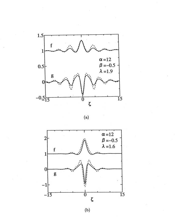
find such numerical solutions for large positivewhen $\alpha=12$ and $\beta=-0.5\mathrm{a}\mathrm{l}\mathrm{e}$ taken, Figs. 2 show the comparison between analytical (broken
lines) and numerical (solid lines) results where $f$ is of ‘bright’ soliton type, while $g$ of depression
soliton type. In Fig. $2(\mathrm{a})$ for $\lambda=1.9$, the analytical results (brokeri lines) with respect to the peak
amplitudes
are
found to be in fairly good agreement with the numerical ones (solid line-s), whilesome discrepancy between them is found in Fig. $2(\mathrm{b})$ for $\lambda=1.6$
.
Furthermore, in both figuresFigs. $2(\mathrm{a})$ and $2(\mathrm{b})$, the analytical results with respect to the oscillatory parts do not agree well
with the numerical ones.
Inref. 1, numerical solutions ofenvelopeshock type in$f$
are
found. However, analytical solutionsof this type could not be obtained in the procedure of the normal form analysis, since we consider
the weakly nonlinearwaves which bifurcat$e$ from linear modulational waves on $|f|=C,$$g=0$
.
\S 4. Concluding remarks
In the preceding section, we
have
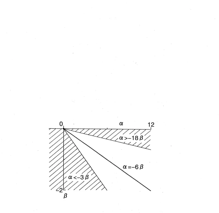
shown the analytical solutions when $q_{0},$$q_{1}<0$ for $\beta,$$\mu<0$.Since $q_{0}<0$ is always satisfied for $\beta<0$, the solitary waves can exist for either $\alpha>-18\beta$ or $\alpha<-3\beta$ from the condition of $q_{1}<0$ in $(3.12_{\mathrm{C}})$. Thus, the solutions can always exist for
$\alpha\leq 0,$$\beta<0$ which corresponds to the capillary-gravity waves. Onthe other hand, integrability of
the resonant system has been examined through the Painlev\’e test.1,17) It is shown that eq. (1.1)
does not pass thePainlev\’e PDE testexcept for $\alpha=\beta=0$, while the reduced equations (3.2) does
pass the Painlev\’e ODE test only for $\alpha+6\beta=0$ when $C\neq 0$. These situations
are
summarized inFig. 3, where the hatched region in the $(\alpha, \beta)$ parameter space shows the existence region of the
solitary waves, while the results of the PDE and ODE tests are, respectively, shownon the closed
circle andonthe solid line. Resultingfromthis, in the hatched region, oursystem is not integrable,
at least, in the
sense
ofPainlev\’e, whichmeans
that the oscillatory solitarywaves
will not have thesoliton properties.
Appendix:
The leading order in the representations of $D$ and $E$ is found to be $O(|A|^{3}, |B|^{3})\mathrm{f}\mathrm{i}^{\backslash }\mathrm{o}\mathrm{m}(3.8)$
and (3.9), while it is $O(|A|^{2}, |B|^{2})$ from (3.7) and (3.11). Therefore, setting all the coefficients
of quadratic terms of $A$ and $B$ in (3.7) to be vanished, the following coefficients in (3.11) are
obtained:
$b_{0}=[-+ \frac{7\beta}{3,8\frac)\beta)9vp_{4})})\frac{\frac{\sqrt{-2\beta}}{\frac c_{1}I\frac(C^{2}\mathrm{i}\sqrt{-}C^{2}\mathrm{i}\zeta}\frac{m_{13}(}{K102\beta}}{\beta^{2}C}+\frac{(\frac{\mathrm{o}^{\ulcorner}\alpha}{\ulcorner 72\alpha}()}{m8\beta 04\ulcorner\beta\alpha(\frac{\alpha}{6}}++\frac{1}{1}]$, $b_{1}=[ \frac{\sqrt{-2\beta}}{C^{2}}(\frac{3\alpha}{}+\frac{19}{8})-\frac{1}{C^{2}}(\frac{8\beta 0\alpha}{2\beta,0}+3)]$;
$c_{\mathrm{O}}=[-- \frac{\mathrm{i}}{C\mathrm{f},\frac{1I}{C}}\frac{\mathrm{o}^{\ulcorner}\alpha}{108\beta}+\frac{1}{)36})\frac{\mathrm{i}\frac{\sqrt{-}(}{\sqrt-2\beta^{2}C}}{\beta^{2}C}\frac{m_{7\alpha}(}{\beta 108\beta I\zeta_{m}2\beta}+_{\overline{36}}\mathrm{t}\ulcorner)$ $]$ ,
$d_{1}=$
.
Using the abovecoefficients, comparisonbetween (3.7) and (3.8) withrespect tothe cubicnonlinear
terms of$A$ and $B$ leads to the coefficients
$p_{1},p_{2},$$q_{1}$ and $q_{2}$.
1) T. Yoshinaga and T. Kakutani: J. Phys. Soc. Jpn. 63 (1994) 445.
2) T. Kawahara, N. Sugimoto and T. Kakutani: J. Phys. Soc. Jpn. 39 (1975) 1379.
3) V. D. Djordjevic and L. G. Redekoop: J. Fluid Mech. 79 (1977) 703.
4) V. E. Zakharov: Sov. Phys. JETP 72 (1972) 908.
5) N. Nishikawa, H. Hojo, K. Mima andH. Ikeji: Phys. Rev. Lett. 33 (1974) 148.
6) see the references cited in ref. 1.
7) T. Kawahara: J. Phys. Soc. Jpll. 33 (1972) 260.
8) M. S. Longuet-Higgins: J. Fluid Mech. 200 (1989) 451.
9) J. -M. Vanden-Broeckand F. Dias: J. Fluid Mech. 240 (1992) 549.
10) T. R. Akylas, Phys. Fluids A5 (1993) 789.
11) M. S. Longuet-Higgins: J. Fluid Mech. 252 (1993) 703.
12) F. Dias and G. Iooss: Physica$\mathrm{D}65$ (1993) 399.
13) G. Iooss and Kirchig\"assner: C. R. Acad. Sci. Paris 311 I (1990) 265.
14) G. Iooss and M. Adelmeyer, Topics in Bifurcation Theory and Applications, Advanced Series in Nonlinear Dynamics (WorldScience, Singapore, 1992) Vol. 3.
15) R. Grimshaw, B. Malomed and E. Benilov: Physica$\mathrm{D}77$(1994)473. 16) T. Yoshinaga, M. Wakamiya and T. Kakutani: Phys. Fluids A3 (1991) 83.
(a)
(b)
Fig. 1. Comparisonbetween analytical (broken lines)and numerical (solid lines) profiles of the oscillatory solitary wavesfor (a) $\lambda=1.9$and (b) $\lambda=1.6$, inwhich$\alpha=-2,$ $\beta=-0.5$and$C=1$,and –sign $\mathrm{o}\mathrm{f}\pm \mathrm{s}\mathrm{i}\mathrm{g}\mathrm{n}\mathrm{s}$ in eq. (3.17)
(a)
(b)
Fig. 2. Comparison between analytical (broken lines) andnumerical (solid lines) profiles of the oscillatory solitary waves for (a) $\lambda=1.9$and (b) $\lambda=1.6$, in which $\alpha=12,$ $\beta=-0.5$ and$C=1,$ $\mathrm{a}\mathrm{n}\mathrm{d}+\mathrm{s}\mathrm{i}\mathrm{g}\mathrm{n}\mathrm{o}\mathrm{f}\pm \mathrm{s}\mathrm{i}\mathrm{g}\mathrm{n}\mathrm{s}$ in eq. (3.17)
Fig. 3. Parameterregion of$\alpha$and$\beta$, where analytical solitarywavesolutions (3.17) canexist in the hatched region,
while eq. (1.1) passes the Painlev\’e PDEteston the closed circle $(\cdot)$ and eq. (3.2) passes thePainlev\’e ODE test