Risk Assessment for Generation Investment by
Random NPV Probit Model based on UNPV Method
Hajime Miyauchi
*and
Tetsuya Misawa
**Abstract
Following the deregulation of the electric power industry, uncertainties such as volatilities in the demand and price of electric power and fuel have increased. It is therefore neces-sary to develop a new method to evaluate investment risks. We have previously devel-oped a risk assessment method using utility indifference net present value (UNPV method). Though identifying the utility function used in the UNPV method is difficult, we propose a “probit” type statistical model to evaluate the investments. The model is derived from a simplification of the UNPV method, and is provided as a type of regression equation for the statistical moments of random net present value (RNPV). We compose a probit model for investment evaluation of a gas thermal power plant project, and compare the results of the UNPV method and the proposed probit model to examine the effectiveness of the proposed probit model.
Index Terms : expected utility theory, generation, investment evaluation, Monte Carlo method, natural gas, power system economics, probit model, random net present value, risk, utility indifference pricing
OIKONOMIKA Vol. 54 No. 1,2017,pp. 75―89
This work is partially supported by Grant-in-Aid for Scientific Research (C) 24540136, (C) 15K04933, and (C) 15K05946, Japan Society for the Promotion of Science (JSPS).
* H. Miyauchi works with Department of Computer Science and Electrical Engineering, Graduate School of Science and Technology, Kumamoto University, 2―39―1 Kurokami, Chuo-ku, Kumamoto, 860―8555, Japan.
E-mail: [email protected]
** T. Misawa works with Graduate School of Economics, Nagoya City University, 1 Yamanohata, Mizuho-cho, Mizuho-ku, Nagoya 467―8501, Japan.
1.INTRODUCTION
Recently, deregulation and reform in the electric power industry have progressed in many parts of the world. This new framework has resulted in the introduction of competi-tion to the electric power generacompeti-tion and retail sectors, as well as open access to electric power networks. Pre deregulation, minimization of total costs was the primary objective when investing in generators. However, post deregulation, profit maximization, especially considering future uncertainties, has become increasingly important. In order to react to these future uncertainties and market risks in a competitive environment, an effective meth-od to determine required investment levels in generation assets needs to be developed. The revenue from generation assets must be estimated properly on the basis of long-term fore-casts of both demand and market price, as well as investors’ attitudes toward expected risks.
Discounted Cash Flow (DCF) method is a well-known approach to assess project value[1]. Net Present Value (NPV) used in DCF method, however, has a limitation in that “random complexities” of cash flow caused by various future uncertainties are not sufficiently ac-counted for; hence, this approach does not provide investors with a suitable evaluation of a project’s risks.
To overcome this limitation, a project assessment method based on “utility indifference pricing” of the expected utility theory has been proposed. This is called the utility indiffer-ence net present value (UNPV) method[2]. The UNPV method employs a utility function to evaluate investor attitude toward risk. The utility function presents investors’ degree of satisfaction upon investing a unit of their property. We have previously applied the UNPV method to assess oil thermal generation projects[3]
. However, because the utility function is not familiar to engineers, it is difficult to identify the utility function’s parameters.
To avoid using the utility function, we have proposed a “probit model”[4]
derived from a simplification of UNPV methods[5,6]. The model is outlined as follows: when we pay atten-tion only to the investment’s execuatten-tion, the project can be expressed by a binary variable, that is, execution or rejection. The probit model is given as a type of regression equation in which dependent variable and explanatory valuables are a project’s binary variable and sev-eral order moments of “random net present values (RNPV).” We estimate the model by as-sessing gas thermal power plant projects considering only fuel and electricity price uncer-tainty[5]. Price uncertainty is simply represented by the mean reverting model with probabilistic variables. We obtain good results from a second-order probit model, using
av-erage and variance of RNPV as explanatory variables.
This paper investigates the effectiveness of our probit model approach under more real-istic price models. To make the uncertainty price models more realreal-istic, we consider “price spikes.” To sufficiently evaluate a project’s execution, we extend the second-order probit model to a fourth-order model. By comparing the statistical results of these two probit mod-els, we investigate the new probit model’s effectiveness.
2.UNPV METHOD
2.1 Net Present Value Method
It is assumed that the time series of future cash flows X={Xn, −1, 2, …,N} is obtained
from the project annually. Let be a random present value obtained from one trial, which is defined as (1).
(1)
where is the designated year and is the discount rate. The present value is given by the expectation of . That is,
( )= [ ( )] (2)
where [・] denotes the expectation. Thus, within the framework of the ordinary NPV method, the randomness of is treated only as the mean value. represents the genera-tion unit’s construcgenera-tion cost, that is, the capital investment, the is calculated by (3).
( )= ( )− (3)
In the conventional NPV, a project is executed if > 0.
Remark 2.1 :
Miyahara[7] has shown that UNPV corresponds to a “risk sensitive measure,” therefore satisfying some suitable and reasonable characters as an evaluation tool for uncertain proj-ects. The measure is called a risk sensitive value measure (RSVM). Recently, some funda-mental studies and applications on RSVM have been proposed[14 ― 17]
.
2.2 Utility Indifference Net Present Value Method[2]
[(− + )]=(0)=0 (4)
where ( ) is the utility function with (0)=0. Utility function ( ) presents investors’ de-gree of satisfaction when they invest their property . The value of return as the “utility indifference price” is defined by the value of v. This means that the expected return equals 0 if investors pay the value of v for the right to obtain uncertain return ; in this context, and v are balanced.
As most investors of electricity generation assets seek to avoid risk, ( ) is assumed to be a risk-aversion type expressed by (5).
u(x)=(1−exp(−βx))/β (5)
where β is a positive constant. On the contrary, when the utility function is given by u(x)=x, it is a risk-neutral type.
To evaluate the project’s uncertain return, which is given as the difference between and construction cost , we substitute ( )= ( )− for in (4) and obtain
(6).
[u(−v+ ( ))]=0 (6)
The value of v satisfying (6) is referred to as the UNPV. In our framework, a project is executed if v>0 instead of >0. Note that if u(x)=x, that is, the risk-neutral type, UNPV v coincides with .
3 RNPV PROBIT MODEL
To calculate UNPV, that is, to calculate the expected value using (6), we employ a Monte Carlo method and obtain sufficient .
Using sufficient , we calculate average [ ] and variance ( ). More-over, we determine the outcome̶execution or rejection̶by UNPV v. Then, UNPV v is transformed to a binary variable as follows:
if v>0, then =1,
(7)
if v 0, then =0.
represents the project’s execution or rejection. Thus, a set of variables { , E[ ], V( )} is obtained. Note that on changing the simulation’s conditions, we obtain other sets of these variables. Moreover,[6] derives a regression equation simplifying UNPV, which is estimated by using many sample sets. is the dependent variable, while the average E [ ] and variance V( ) are explanatory variables. That is,
= 0+ 1[ ] 2( ) (8) where 0,1,2 are regression coefficients obtained by the maximum likelihood estimation under the assumption that the estimation error in (8) is a Gaussian distribution. The model in (8) is called the second-order RNPV probit model. To assess the project, the average val-ue and the variance of are substituted in (8). If >0, the project is executed. When a distribution of is a Gaussian distribution, (6) can be mathematically con-verted to (8) without the interception term 0. However, the resulting distributions of
are not Gaussian distributions because of price spike in fuel and electricity prices. To derive a more accurate probit model, a higher-order term should be employed. We use the third- and fourth-order central moments of . That is,
= 0+ 1[ ] 2( ) + 3[( − [ ]) 3 ] (9) + 4[( − [ ]) 4 ] The model in (9) is called the fourth-order RNPV probit model.
If the distribution of the estimation error in (8) or (9) is of the logistic type, we can obtain the second or fourth order RNPV “logit” model[6]
.
4 SIMULATION MODEL
4.1 Expression of Prices
This section applies the UNPV method and simplified RNPV probit model toward the in-vestment in a gas thermal power plant.
Under a deregulated regime, the electric power industry poses significant risks. Howev-er, to simplify our simulation, we consider only wholesale electricity and natural gas price fluctuations in the market. We ignore other uncertainties, such as trading volume, bidding strategy, and transmission congestion. We consider only the cost of fuel to generate elec-tricity, ignoring start-up costs.
Annual profit for the time series of cash flow { , =1, 2,…, } is given by (10).
(10)
where and i are the daily average prices of electricity and natural gas on day ,
re-spectively. * is the conversion rate, which will be explained in the next section. To simpli-fy the simulation, it is assumed that the generator operates for 14 hours a day. Accordingly,
=14( − *
・ ) is the cash flow per day. Annual profit is the difference between the total profit of one year and the operating maintenance cost as shown in (10). The daily average prices of electricity and natural gas, and , respectively, are as-sumed to be described by the mean reverting models fluctuated by random numbers ac-cording to the Gaussian distribution[8]
.
(11)
(12)
where, α, σ, and Δt are mean regressive rate, volatility, and time interval, respectively, and εi
is a series of normal random numbers. The constant μ is defined as μ=In( ), where is the long-term price level. Subscripts 1 and 2 of σ and εi in (11) and (12) denote the
parame-ters concerning the price of electricity and natural gas, respectively. We assume the ran-dom numbers of electricity and gas prices, ε1, i and ε2, i, respectively, as being statistically in-dependent.
When we consider price spike, the prices obtained by (11) or (12) is multiplied by price spike magnification s according to the price spike probability s .
4.2 Simulation Method and Parameters
Using appropriate values of long-term price level , mean regressive rate α, and volatility
σ, we employ a Monte Carlo method to attain many values. We run 20,000 trials for cases without price spikes, and 50,000 trials for cases with price spikes using the Monte Car-lo method. UNPV v is then calculated using (6) and converted to the binary variable as mentioned in Sec. III. Thus, we can obtain one set of variables { , [ ], ( )}. Changing parameters , α, and σ, we repeatedly run the Monte Carlo method to obtain many sets of variables{ [ ] ( )}. From these sets, we obtain the probit model as mentioned in Sec. III.
All parameters except , α, and σ used in the simulation are listed in Table I.
TABLE Ⅰ SIMULATION PARAMETERS
Δt [year] 1/365 0.03 [year] 22 [JPY/kW] 2.0* 105 [JPY/(kW・year)] 9636
The conversion rate *
is defined as follows: the calorific value of natural gas is approxi-mately 1 MMBtu=252×10 3 kcal. Assuming a generating efficiency of 43% and an exchange rate of 1 USD=100 JPY, we can calculate *
[(JPY/MMBtu)/(USD/kWh)] using 1 kWh= 860kcal.
(13)
5 RESULTS OF UNPV
5.1 Cases without Price Spike
The electricity price parameters , α, and σ are based on the system price data of JEPX[9]. Natural gas price parameters are based on the price of Hunny Hub[10]
.
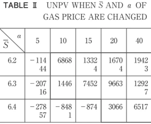
Table II shows a section of the UNPV simulation results considering uncertainty only in natural gas prices without the price spike. Concerning the other parameters except for those listed in Tables I and II, volatility σ of natural gas price is set at 1.0. Parameters [JPY/kWh], α, and σ of electricity price are set at 9.5, 110 and 3.3, respectively.
TABLE Ⅱ UNPV WHEN ‾ AND α OF GAS PRICE ARE CHANGED
α 5 10 15 20 40 6.2 −114 44 6868 1332 4 1670 4 1942 3 6.3 −207 16 1446 7452 9663 1292 7 6.4 −278 57 −848 1 −874 3066 6517
On the right side surrounding bold lines in Table II, the project is evaluated to determine if it should be executed under these conditions, as UNPV is positive. On the contrary, the project should not be executed in the conditions given on the left side.
We calculated 47 and 60 cases considering uncertainties in electricity prices and natural gas prices, respectively. In addition, 255 cases were simulated considering uncertainties in both electricity and natural gas prices. Thus, we calculated 362 cases in total. The parame-ters , α, and σ for electricity prices fluctuated in the range of 9.0 ― 10.3, 70 ― 160, and 2.5 ― 39,
respectively. The parameters , α, and σ for natural gas price fluctuated in the range of 5.7 ― 6.5, 5 ― 40, and 0.5 ― 2.0, respectively. Based on JEPX and Hunny Hub prices, these value rang-es selected as the UNPV rrang-esults are split into positive or negative, that is, project execution or rejection.
5.2 Cases with Price Spike
Cases of price spikes for electricity and/or natural gas are considered. A price spike is generated at constant probability s with no relation to time series. During a price spike, the average price during the entire day is assumed to jump by a certain constant magnifica-tion s .
Table III shows a segment of the UNPV simulation results considering uncertainty only in natural gas prices with the price spike. Natural gas price volatility σ is set at 1.0, and the pa-rameters of price spike s and s are set at 2 and 0.1% , respectively. Moreover, in Table II, parameters [JPY/kWh], α, and σ of electricity price are set at 9.5, 110 and 3.3, respectively.
TABLE Ⅲ UNPV WHEN ‾ AND α OF GAS PRICE ARE CHANGED WITH PRICE SPIKES
α 10 15 20 25 30 6.0 717 1180 0 1962 4 2359 7 2568 4 6.2 −135 99 −215 3 6031 1056 3 1235 4
UNPV here is lower than the results shown in Table II as the natural gas price, that is, the fuel price, is higher than the cases in Table II due to the price spike.
We simulated 240 cases with price spikes in electricity and/or natural gas prices. The price parameters , α, and σ of electricity and natural gas fluctuated, as in the previous sec-tion. Concerning price spike parameters, probability s and magnification s fluctuated in the range of 0.1% ― 5% and 2 ― 10, respectively.
6 RESULTS OF RNPV PROBIT MODEL
6.1 Cases without Price Spikes
Using the results from the 362 cases in Sec. V- , the second-order RNPV probit model (8) is derived. The obtained RNPV probit model with interception is shown in (14), while (15) shows the model without interception.
=−2.124+4.29×10⁻⁴[ ]−1.21×10⁻⁷( )
(−4.641) (6.622) (−6.480) (14)
= 2.458×10⁻⁴[ ]−8.81×10⁻⁸( )
(7.987) (−7.702) (15)
The t-ratio values are shown in parentheses under each regression coefficient.
The fourth-order RNPV probit model shown in (9) is also derived. The obtained probit model is shown in (16) and (17). The t-ratios for (16) and (17) are listed in Table IV.
=−1.694+5.220×10⁻⁴ [ ]−1.766×10⁻⁷ ( ) −9.484×10⁻¹² [( − [ ])3 ] +3.153×10⁻¹⁷ [( − [ ])4 ] (16) = 3.824×10⁻⁴ [ ]−1.481×10⁻⁷ ( ) −1.388×10⁻¹¹[( − [ ])3] +1.142×10⁻¹⁷ [( − [ ])4 ] (17)
Table IV shows the comparison between the second-order and fourth-order RNPV probit models. From top to bottom, it shows the number of incorrect results of the RNPV probit model from UNPV results, the proportion R/N which adheres to both results, the t-ratio for regression coefficients of interception, average E[ ], variance V( ), third- and fourth-order terms, and Wald test statistics.
TABLE Ⅳ RESULTS OF RNPV PROBIT
MODEL (WITHOUT PRICE SPIKES)
second-order model fourth-order model interception With with out with with out Fault 14 24 13 18 R/N 96.1% 93.4% 96.4% 95.0%
t-ratio −4.6 41 −3.8 43 6.62 2 7.98 7 6.22 8 6.76 7 −6.4 80 −7.7 02 −5.8 32 −6.4 89 −0.6 76 −1.0 59 0.74 9 0.29 8 Wald 44.2 5 63.8 3 39.6 3 46.5 8
The assessment of whether to execute or reject a project on the basis of the proposed probit model is almost the same as results based on the UNPV method. As described above, identifying the parameters of the utility function is difficult. However, this result in-dicates that the utility function is not necessary if sufficient information from the results of project assessment is available. Using these results, we can determine the RNPV probit model and assess the project by the probit model.
T-ratio absolute values, with the exception of the higher-order terms determined in Table IV, are larger than 2.59, which is the value of 1 percentage point of the t-distribution. More-over, the Wald test values are larger than 9.21, which is the value of 1 percentage point of the x2 distribution. Therefore, we conclude that all explanatory variables except those for higher-order terms are significant. Higher-order terms, however, are not significant, indicat-ing that the regression equation does not require these higher-order terms as explanatory variables. That is, the second-order RNPV probit model is sufficient for cases without price spikes.
Finally, as previously mentioned, the interception is not theoretically required when an distribution is a Gaussian distribution[6]. However, the difference between and Gaussian distributions requires the intercept to suppress the error.
6.2 Cases with Price Spikes
Using the results from 240 cases from Sec. V- , the second-order RNPV probit model shown in (8) is derived. The obtained probit model with interception is shown in (18), while that without interception is shown in (19).
=−0.728+3.21×10⁻⁴[ ]−1.20×10⁻⁷( )
= 2.91×10⁻⁴
[ ]−1.20×10⁻⁷
( )
(6.458) (−6.316) (19)
The fourth-order RNPV probit model in (9) is derived. The obtained probit model is shown in (20) and (21), and t-ratios of (20) and (21) are listed in Table V.
=−0.761+9.197×10⁻⁴ [ ]−4.410×10⁻⁷ ( ) +7.237×10⁻¹¹[( − [ ])3] +7.215×10⁻¹⁶ [( − [ ])4 ] (20) = 8.623×10⁻⁴[ ]−4.330×10⁻⁷( ) −6.941×10⁻¹¹ [( − [ ])3 ] +6.956×10⁻¹⁶[( − [ ])4] (21)
Table V shows the comparison between the second-order and fourth-order RNPV probit models. From top to bottom, Table V lists the number of incorrect results of the RNPV pro-bit model from UNPV results, the proportion of R/N that adheres to both results, the t-ratio for the regression coefficients of interception, the average E[ ], the variance V( ), the third- and fourth-order terms, and the Wald test statistic.
TABLE Ⅴ RESULTS OF RNPV PROBIT
MODEL (WITH PRICE SPIKES)
second-order model fourth-order model interception with with out With with out Fault 13 14 6 7 R/N 94.58% 94.17% 97.50% 97.08% t-ratio −1.94 8 −1.14 7 6.264 6.458 4.117 4.090 −5.79 1 −6.31 6 −4.11 0 −4.09 2 3.533 3.335 3.870 3.725 Wald 39.33 41.70 17.34 17.85
The Wald test shows the significant explanatory variables, and the t-ratio, with the ex-ception of the interex-ception, shows the significant explanatory variables. Especially, the third- and fourth-order terms in the fourth-order RNPV probit model are significant,
indicat-ing that the regression equation requires these higher-order terms as explanatory variables. The assessment of whether to execute or reject a project on the basis of the proposed probit model is almost the same as results based on the UNPV method as well as the cases without price spikes. The error of the fourth-order RNPV probit model from the UNPV is smaller than that of the second-order RNPV probit model. Therefore, the fourth-order RNPV probit model is effective for cases with price spikes.
Finally, the t-ratio of the interception is smaller than the value of 1 percentage point of the t-distribution. Though we think the interception term is used for the difference in the and Gaussian distributions, the price spike is thought to comprise much of a differ-ence between the and Gaussian distributions. We hypothesize that the significance of interception becomes relatively lower because the higher-order term has larger signifi-cance. The exact resolution of this discrepancy will be addressed in our future work.
6.3 RNPV Probit Model by All Cases
Finally, using the results of all 602 cases (=362cases without price spikes+240cases with price spikes), the second-order RNPV probit model in (8) is derived. The obtained probit model with interception is given in (22), while that without interception is given in (23)
=−1.455+3.31×10⁻⁴[ ]−1.00×10⁻⁸( )
(−5.328) (9.553) (−8.758) (22)
=2.37×10⁻⁴[ ]−8.99×10⁻⁸( )
(10.64) (−10.27) (23)
The fourth-order RNPV probit model in (9) is also derived. The obtained probit model is shown in (24) and (25), and t-ratios of (24) and (25) are listed in Table VI.
=−1.565+5.071×10⁻⁴[ ]−1.852×10⁻⁷( ) +2.568×10⁻¹¹ [( − [ ])3 ] +1.331×10⁻¹⁶[( − [ ])4] (24) =3.733×10⁻⁴ [ ]−1.586×10⁻⁷ ( ) +1.933×10⁻¹¹[( − [ ])3] +1.083×10⁻¹⁶ [( − [ ])4 ] (25)
Table VI shows a comparison between the second-order and fourth-order RNPV probit models. From top to bottom, Table VI shows the number of incorrect results of the probit model from UNPV results, the proportion of R/N that adheres to both results, the t-ratio for the regression coefficients of interception, the average E[ ], the variance V( ),
the third- and fourth-order terms, and the Wald test statistic, as well as Tables IV and V.
TABLE Ⅵ RESULTS OF RNPV PROBIT
MODEL (ALL 602 CASES)
second-order model
fourth-order model interception
with with out with with out
Fault 31 40 20 26 R/N 94.85% 93.36% 96.86% 95.68% t-ratio −5.32 8 −4.60 9 9.553 10.64 8.195 8.982 −8.75 8 −10.2 7 −8.04 1 −8.87 9 4.479 4.157 6.264 6.438 Wald 91.42 113.1 68.33 81.31
The Wald test and t-ratios show all explanatory variables to be significant. The error of the fourth-order RNPV probit model from the UNPV is smaller than the one in the second-order RNPV probit model shown in Table V. Therefore, the fourth-second-order RNPV probit model is effective in all cases, with or without price spikes.
7 CONCLUSION
We had previously proposed a risk assessment method for generation investment with various uncertainties by using a probit model described by the moments of RNPV. On hav-ing sufficient information regardhav-ing a project’s assessment results, that is, execution or re-jection, as well as the average and variance of the NPV, the probit model as a regression equation can be determined. In this paper, we apply the probit model to assess a gas ther-mal power plant project. We investigate the effectiveness of the proposed probit model un-der more realistic price models. Though uncertainties only in electricity and natural gas prices are assumed, we calculate 362 cases without price spikes and 240 cases with price spikes under different conditions. From the results of these cases, we derive the RNPV pro-bit model and compare it with the results from the UNPV method which is the origin of our
statistical model. Moreover, we prepare two probit models, a second-order RNPV probit model, in which explanatory variables include the average and variance of , and a fourth-order RNPV probit model, in which explanatory variables include the average, vari-ance, and the third- and fourth-order central moments. According to our results, the probit model is mostly consistent with the UNPV method for risk-averse investors. If project as-sessment data does not include price spikes, the second-order RNPV probit model is suffi-cient. However, if the data includes price spikes, the use of the fourth-order RNPV probit model is required, as proposed in this paper, to represent the difference between the RNPV and Gaussian distributions.
These results indicate that risk-averse investors can directly apply our probit model to practical project evaluations without using the UNPV method. The procedure for such an evaluation is outlined as follows:
(a) The investor prepares ahead of time the assessment results for execution or rejection to-gether with the RNPV moments obtained by simulation data using various scenarios. (b) Using the results, the second- or fourth-order RNPV probit model is derived from the maximum likelihood estimation.
(c) On the basis of another scenario simulation, the investor obtains sample RNPV values for the new project under evaluation, and calculates the moments of RNPV for the project. (d) Finally, the investor substitutes the moments from (c) into the RNPV probit model ob-tained in (b), and determines execution or rejection of the new project based on the model’s signature.
The probit model theory can be developed in various forms[4]
, and we have already pro-posed an extension of the model to a three-level ordered probit model[11], and an application to assessment of a project’s execution probability[12,13]
. We can easily extend these results to the case of logit model. On the other hand, we must actually show our method’s applicabili-ty an application to a practical problem.
ACKNOWLEDGMENTS
We would like to thank Honorary Prof. Y. Miyahara of Nagoya City University, Nagoya Japan, for his informative suggestions. We also thank Mr. N. Hirata, a graduate student of Kumamoto University, for his great contribution to this study.
[1] R. Brealey, S. Myers, G. Sick, and R. Whaley , “Principles of Corporate Finance,” McGraw-Hill 2007.
[2] Y. Miyahara, “Project assessment method b a s e d o n t h e e x p e c t e d u t i l i t y t h e o r y , ” Discussion Papers in Economics, No. 446, Nagoya City University, 2006 ( ). [3] H. Miyauchi., K. Miyahara, T. Misawa, and K.
Okada, “Risk assessment for generation investment based on utility indifference p r i c i n g , ” P r o c e e d i n g s o f C I G R E O s a k a Symposium, 405, November 2007.
[4] R. Davidson and J. MacKinnon, “Estimation and Inference in Econometrics,” Oxford Univ. Press, 1993.
[5] N. Hirata, H. Miyauchi, and T. Misawa, “Composition of probit model of simplified UNPV method,” Proc. of 16th International Conference on Electrical Engineering, PM ― 01, July 2010.
[6] T. Misawa, “Simplification of utility indifference net present value method,” OIKONOMIKA, vol. 46, No. 3, pp. 123 ― 135, 2010.
[7] Y. Miyahara, “Risk-sensitive value measure method for projects evaluation,” Journal of Real Options and Strategy, vol. 3, pp. 185 ― 204, 2010. [8] L . C l e w l o w a n d C . S t r i c k l a n d , “ E n e r g y
Derivatives Pricing and Risk Management,” Sigmabase Capital, 2004.
[9] Japan Electric Power Exchange (JEPX), “System price data” [Online]. Available: http:// www.jepx.org/
[10] International Exchange, “Global commodity markets” [Online]. Available: http://www. theice.com/
[11] J. Sakaguchi, H. Miyauchi, and T. Misawa, “Risk assessment of power plant investment by three level ordered probit model considering project suspension,” Proc. of 2013 IREP Symposium, 2013.
[12] T. Hirose, H. Miyauchi, and T. Misawa, “Project value assessment of thermal power plant based on RNPV probit model considering real options,” Journal of Real Options and Strategy, vol. 5, pp. 1 ― 18, 2012 ( ).
[13] M. Hayashida, H. Miyauchi and T. Misawa , “Asset Evaluation of Thermal Power Plant Project by Probit Model”, Proceedings of 20 th
I n t e r n a t i o n a l C o n f e r e n c e o n E l e c t r i c a l Engineering (ICEE 2014), vol. PSO ― 2004, pp. 666 ― 670, 2014.
[14] Y. Miyahara, “Scale risk and its valuation”, OIKONOMIKA, Nagoya City University, vol. 49, pp. 45 ― 56, 2013 (in Japanese).
[15] Y. Miyahara, “Evaluation of the scale risk”, RIMS Kokyuroku, Research Institute of Mathematical Sciences, Kyoto University, vol. 1886, pp. 181 ― 188, 2014.
[16] Y. Ide, H. Miyauchi and T. Misawa, “Value assessment of power generation project by UNPV method considering scale effects”, Proceedings of 2014 Makassar International Conference on Electrical Engineering and Informatics, MICEEL 2014, pp. 23 ― 27, 2014. [17] L. Ban, T. Misawa and Y. Miyahara, “Valuation
of Hong Kong REIT based on Risk Sensitive Value Measure Method”, International Journal of Real Options and Strategy, vol. 4, pp. 1 ― 33 (2016).