系統樹最節約復元束の完備分配性について
-Lattice-theoretic
propertiesof
MPR-posets inphylogeny-電気通信大学大学院 宮川幹平(Kampei Miyakawa)
東海大学高輪短期大学部 成嶋弘 (Hiroshi Narushima)
On the background of biology such as taxonomy, cladistics and phylogeny, the principle of
maximum parsimony also called Wagner Parsimonyhasbeen mathematically formulatedand then
amathematical and algorithmic theory has been$\mathrm{d}\mathrm{e}\mathrm{v}\mathrm{e}\mathrm{l}\mathrm{o}\mathrm{P}\mathrm{i}\mathrm{n}\mathrm{g}[2-12]$. The principle
assumes
that thetotal amount of evolutionary changesis globally minimized. The problems and related problems
on this minimization have been called the Most-Parsimonious Reconstruction (abbreviated to
MPR) Problems in phylogeny.
In Narushima [8], the MPR Problems are classified into two kinds of topics. One is called
the First MPR Problem “given a phylogenetic tree with the external nodes (which express the
operational taxonomic units) of which characters are stated, find an assignment of
character-states to all internal nodes (which express the hypothetical taxonomic units) of the tree, so as
to minimize the length (the total amount of evolutionary changes) of the tree.” This is also
known as “the character-state minimization.” The other is the Second MPR Problem (or the
WagnerTree Problem) “givenaset of operational taxonomic units of which characters arestated,
find a phylogenetic tree with the set as the external nodes, and simultaneously an assignment of
character-states to all internal nodes of the tree, so as to minimize the length of the tree.” Such
an optimal phylogenetic tree is called a Wagner tree. It is well-known that the latter problem
is strongly related to the Steiner Problem in Phylogeny (SPP) and the Rectilinear Steiner Tree
(RST) problem etc. Both problems described above originate in Farris [2]. In this paper, we
discuss the former problem under linearly ordered character-states, that is, in the framework
based on the method of Hanazawa, Narushima and $\mathrm{M}\mathrm{i}\mathrm{n}\mathrm{a}\mathrm{k}\mathrm{a}[3]$
.
We use the notation in [3, 6, 9, 10]. In this paper, let the set $\Omega$ oflinearly ordered
character-states be the set $\mathrm{R}$ of real numbers unless otherwise stated, because we discussthe completeness
of posets, introduced later. Let $\Omega^{n}$ denote the $\mathrm{n}$-dimensional Cartesian product of $\Omega$. Let $T=$
(V,$E,$$\sigma$) be any undirected simple tree whose endnodes are evaluated by a weight function a :
$V_{O}arrow\Omega^{n}$, which is called a multi-character state function, where $V$ is the set of nodes, $V_{O}$ is
the set of endnodes, $V_{H}$ is the set of internal nodes, and $E$ is the set of branches. Note that
$V_{O}\cup V_{H}=V$ and $V_{O}\cap V_{H}=\emptyset$
.
We call this tree an $el$-tree. For an $\mathrm{e}1$-tree $T$, we define anassignment $\lambda$ : $Varrow\Omega^{n}$ such that $\lambda|V_{O}$ (the restriction of $\lambda$ to $V_{O}$)
$=\sigma$, where $\lambda(u)$ is called
a state of $u$ under $\lambda$
.
This assignment is called a reconstruction on an $\mathrm{e}1$-tree $T$. We denotethe restriction of $\lambda$-range to the i-th component of $\Omega^{n}(1\leq i\leq n)$ by $\lambda_{i}$. For each branch $e$
in $E$ of an $\mathrm{e}1$-tree $T$ with a reconstruction $\lambda$, we define the length $l(e)$ of branch $e=\{u, v\}$ by
$\sum_{i=1}^{n}|\lambda_{i}(u)-\lambda_{i}(v)|$, whichis said to be the Manhattan distance or the rectilinear distance. The
length $L(T|\lambda)$ ofan$\mathrm{e}1$-tree$T$under the reconstruction$\lambda$ is the sumof the lengths ofthe branches.
That is, $L(T| \lambda)=\sum_{e\in E}l(e)$
.
Then we define the minimum length $L^{*}(T)$ of$T$ by$L^{*}(T)= \min$
{
$L(\tau|\lambda)|\lambda$ is a reconstruction on$T$}.
Note that $L^{*}(T)$ is well-defined. A reconstruction $\lambda$ such that $L(T|\lambda)=L^{*}(T)$ is called a
most-parsimonious reconstruction (abbreviatedto MPR) on$T$. Generally, an$\mathrm{e}1$-tree $T$ has more than
oneMPR. Thefollowingisoneof thekeyconcepts in the subject. The set
{
$\lambda(u)|\lambda$ is an MPRon $T$}
ofstates is called the $MPR$-set ofa node $u$ and written as $S_{u}$
.
We here note the followingimportant fact. Considering the definitin of$L(T|\lambda)$, that is,
we see that this minimization allows us to treat each component (character) independently.
In-deed, this independence among characters is a crucial assumption ofour method. So, hereafter,
we treat only the single-character case for an el-tree.
For agiven$\mathrm{e}1$-tree$T=(V, E, \sigma)$, we definea rooted $el$-tree $T^{(r)}$ rooted at any element
$r$ in $V$.
The rooted $\mathrm{e}1$-tree $T^{(r)}$ is simply written $T$ if it is understood. The parent-child relation
$\{u, v\}$
in $E$ onarooted $\mathrm{e}1$-tree $T$is denoted by $uarrow v$
or
$p(v)=u$, whichmeans
$u$ is aparent of$v$ (or $v$
is a child of$u$). For each $u$ and $v$ in $V,$ $u$ is called an ancestor of$v$, written $uarrow v*$, if there is a
sequence of nodes $u=u_{1},$$u_{2},$ $\cdots,$$u_{n}=v$ in $V$ such that $u_{i}arrow u_{i+1}(1\leq i\leq n-1)$. In a rooted
$\mathrm{e}1$-tree, there is only
one
node without a parent, which is called the root, anda
node without a
child is called a
leaf.
For each $u$ in $V$, we denote a subtree ofa rooted $\mathrm{e}1$-tree$T$ induced from asubset $\{u\}\cup\{v\in V|uarrow v\}*$ of$V$ by$T_{u}$, where$u$ is the root. If$r$ is an endnode, i.e., $r\in V_{O}$ and
$s$ is its unique child, we denote the rooted $\mathrm{e}1$-tree $T^{(r)}$ by $(T_{s}, r)$
.
In this case, the subtree$T_{s}$ is
called the body of the tree $T^{(r)}$ ; oherwise, i.e., if
$r\in V_{H}$, the body of$T^{(r)}$ is $T^{(r)}$ itself.
We denote the set $\{1, 2, \cdots, n\}$ of$n$ elements by $[n]$
.
Let $a_{i}(i\in[2n])$ be any elements in $\Omega$,and be sorted in ascending order as follows:
$x_{1}\leq x_{2}\leq\cdots\leq x_{n}\leq x_{n}+1\leq\cdots\leq x_{2n}$.
Then we call $x_{n}$ and $x_{n+1}$ the median two points of the numbers $a_{i}(i\in[2n])$, and denote $\langle x_{n}, x_{n+}1\rangle$ by
$\mathrm{m}\mathrm{e}\mathrm{d}2\langle a_{1,2}a, \cdots, a_{2n}\rangle$ or $\mathrm{m}\mathrm{e}\mathrm{d}2\langle a_{i} :i\in[2n]\rangle$
.
Let $I_{i}(i\in[m])$ be any family of closed intervals in$\Omega$
.
Thenwe denote the median twopoints
ofall the endpoints of$I_{i}(i\in[m])$ by
$\mathrm{m}\mathrm{e}\mathrm{d}2\langle I_{1}, I_{2}, \cdots, I_{m}\rangle$ or $\mathrm{m}\mathrm{e}\mathrm{d}2\langle I_{i} :i\in[m]\rangle$
.
Let $\mathrm{m}\mathrm{e}\mathrm{d}2\langle I_{i} :i\in[m]\rangle=\langle x, y\rangle$
.
Thenwecall the closed interval $[x, y]$ in$\Omega$the median interval of$I_{i}(i\in[m])$, which is the key concept ina
series ofour
papers, and denote it by$\mathrm{m}\mathrm{e}\mathrm{d}\langle I_{1}, I_{2}, \cdots, I_{m}\rangle$ or $\mathrm{m}\mathrm{e}\mathrm{d}\langle I_{i} :i\in[m]\rangle$
.
For each node $u$ in the body of a rooted $\mathrm{e}1$-tree $T$, we assign a closed interval $I(u)$
of $\Omega$
recursively asfollows:
$I(u)=\{$ $[\sigma(u), \sigma(u)]$ if$u$ is a leaf,
$\mathrm{m}\mathrm{e}\mathrm{d}\langle I(v) :u\mapsto v\rangle$ otherwise.
This $I(u)$ is called the characteris$tic$ interval ofa node $u$, andso is $I$ the characteris$tic$ interval
map on$T$
.
Wenowrestatesomeprevious results whicharepaticularly related to newresults stated later.
The following is a qualitative expression of Theorem 1 (Theorem $3(\mathrm{i}\mathrm{i})$) in [3], which shows the
necessary and sufficient condition for areconstruction
on
$T$ to be an MPR on $T$.
This theoremmay be saidto be the fundamental theoremon the first MPRproblem.
Theorem A Let $T$ be a rooted $el$-tree $(T_{s}, r)$ and $\lambda$ be a reconstruction on T. $\lambda$ is an $MPR$ on
$T$
if
and onlyif for
any $u\in V_{H},$ $\lambda(u)\in \mathrm{m}\mathrm{e}\mathrm{d}\langle[\lambda(p(u)), \lambda(p(u))], I(v) : uarrow v\rangle$, where I is thecharacteristic interval map on $T$
.
By using Theorem$\mathrm{A}$, we canrecursivelyobtain all MPRsonagiven$\mathrm{e}1$-tree$T$
.
For details see$[3, 6]$. Thenwe denote the set of MPRs on an $\mathrm{e}1$-tree $T$ by
$\mathrm{R}\mathrm{m}\mathrm{p}(T)$
.
Thefollowing is CorollaryCorollary $\mathrm{B}$ Let
$u$ be any internal node
of
an $el$-tree T. Let I be the characteristic interval mapon a rooted $el$-tree $T^{(u)}$
.
Then $I(u)$ is the $MPR$-set $S_{u}$.From Theorem $\mathrm{A}$,
we
see
that $\mathrm{m}\mathrm{e}\mathrm{d}\langle[\lambda(p(u)), \lambda(p(u))], I(v) :uarrow v\rangle$ is the MPR-set of node $u$under the restriction that an element $\lambda(p(u))$ in $S_{p(u)}$ has been assigned to $u’ \mathrm{s}$ parent $p(u)$. We
denote this subset of the MPR-set $S_{u}$ by $S_{u}|x$. That is,
$S_{u}|x=\mathrm{m}\mathrm{e}\mathrm{d}\langle[x, x], I(v) : uarrow v\rangle$ ,
where $x$ is anelement in $S_{p(u)}$.
The following is Theorem 1 in [6], which gives arecursive characterization for each MPR-set.
Theorem $\mathrm{C}$ Let $T$ be a rooted $el$-tree $(T_{S}, r)$
.
Then each $MPR$-set $S_{u}$for
each internal node $u$of
$T$ is recursively decided by$S_{u}=[ \min(S_{u}|\min(S_{p(u}))), \max(S_{u}|\max(s_{p(u)}))]$
.
Fig. 1: An undirected $\mathrm{e}1$-tree $T$ Fig. 2: All MPR-sets on $T$
Table 1: $\mathrm{R}\mathrm{m}\mathrm{p}(T)$
Since the minimization ofa reconstruction $\lambda$ : $Varrow\Omega$ on an$\mathrm{e}1$-tree$T=(V, E, \sigma)$ is ourcenter
(written as $\triangle$) of $\Omega$
.
Therefore, we may think of the set $\{\lambda : Varrow\triangle\}$ of reconstructions on $T$as the general framework ofour subject. Let $\mathrm{R}\mathrm{e}\mathrm{c}(T)$ denote the set $\{\lambda : Varrow\Delta\}$. Then the
usual ordering $\lambda\leq\mu$ on$\mathrm{R}\mathrm{e}\mathrm{c}(\tau)$ is defined by $\lambda(u)\leq\mu(u)$ for all $u$ in $V$
.
We call $(\mathrm{R}\mathrm{e}\mathrm{C}(\tau), \leq)$ aREC-poset.
On the other hand, from aphylogenetic point ofview, Minaka $[4, 5]$ has introduced the two
partial orderings on $\mathrm{R}\mathrm{m}\mathrm{p}(T)$ to investigate the relationships among MPRs. One is the usual
ordering andthe other is apartial ordering that dependson astate ofaspecified root ofa given
el-tree.
We now give
a
mathematically explicit formulation for those partial orderings. Let $T$ be an$\mathrm{e}1$-tree. The usual ordering $\lambda\leq\mu$ on $\mathrm{R}\mathrm{m}\mathrm{p}(T)$ is defined by $\lambda(u)\leq\mu(u)$ for all $u$ in $V$. Let
$T$ be a rooted $\mathrm{e}1$-tree $(T_{s}, r)$
.
A binary relation$a\leq_{\sigma(r)}b$
on
$\Omega$ is defined by $\sigma(r)\leq a\leq b$ or$\sigma(r)\geq a\geq b$
.
Then abinaryrelation$\lambda\leq_{\sigma(r)\mu}$on$\mathrm{R}\mathrm{m}\mathrm{p}(T)$ is defined by$\lambda(u)\leq_{\sigma(r)\mu}(u)$ forall $u$in $V$. It is easily shown that those relations are partialorderings. $(\mathrm{R}\mathrm{m}\mathrm{p}(\tau), \leq)$is called a usual
MPR-po8et which is really an induced subposet of$(\mathrm{R}\mathrm{e}\mathrm{C}(\tau), \leq)$, and $(\mathrm{R}\mathrm{m}\mathrm{p}(\tau), \leq_{\sigma(r)})$ is called a
$\sigma(r)$-version $MPR$-poset. Note that the usual MPR-poset is uniquely defined for an $\mathrm{e}1$-tree, but
the $\sigma(r)$-version MPR-poset, depending on the character-state ofa specified root, is defined for
each rooted el-tree.
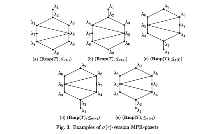
We here illustrate
some
$\sigma(r)$-version MPR-posets in Fig.3 for the $\mathrm{e}1$-tree $T$ in Fig.1. From$\sigma(l)=\sigma(n)=1\leq\lambda(u)(\lambda\in \mathrm{R}\mathrm{m}\mathrm{p}(T), u\in V)$ in Table 1 and the definition of $\sigma(r)$-version
MPR-poset, we see that each $\sigma(r)$-versionMPR-poset of (c) and (d) in Fig.3 is order-isomorphic
to the usual MPR-poset.
$((1’(\iota \mathrm{t}\mathrm{m}\mathrm{p}(^{\mathit{1}}’,\underline{\backslash }\sigma(n))$ $(^{\mathrm{c}}’(^{\iota \mathrm{L}\mathrm{I}\mathrm{I}1}\mathrm{p}(\mathit{1}’,\underline{\backslash }\sigma(_{0))}$
Fig. 3: Examples of$\sigma(r)$-version MPR-posets
It is easily shown that the REC-poset $(\mathrm{R}\mathrm{e}\mathrm{c}(\tau), \leq)$ is a complete distributive lattice. At the
start of investigating the completeness of MPR-posets and the distributivity, that is, whether $‘(\mathrm{a}\mathrm{n}$
MPR-poset is a complete sublattice of the lattice $(\mathrm{R}\mathrm{e}\mathrm{C}(\tau), \leq)$ or not”, in the main section, we
first restate the the following which is Proposition5 in [9].
Proposition $\mathrm{D}$ Let $T$ be an $el$-tree. Let $\lambda_{\max}(\lambda_{\min})$ denote a reconstruction $\lambda$ on$T$ such that
the greatest (least) element
of
the $MPR$-poset $(\mathrm{R}\mathrm{m}\mathrm{p}(\tau), \leq)$.
It is well-known theorem in lattice theory that a lower-complete poset with the greatest
element is a complete lattice. Hence, from Proposition $\mathrm{D}$
we
see that the lower-completeness(upper-completeness) of $(\mathrm{R}\mathrm{m}\mathrm{p}(\tau), \leq)$ is sufficent to show the following, the first main theorem
in this paper.
Theorem 1. Let $T$ be an $el$-tree. Then the usual $MPR$-poset $(\mathrm{R}\mathrm{m}\mathrm{p}(\tau), \leq)$ is a complete
dis-tributive lattice.
We nextinvestigate lattice-theoretic properties of$\sigma(r)$-version MPR-posets. First ofall, recall
that the usual MPR-poset is uniquely defined for an $\mathrm{e}1$-tree, but the $\sigma(r)$-version MPR-poset.
depending onthe character-state ofa specified root, is defined for each rooted $\mathrm{e}1$-tree. The same
framework as usual MPR-posets applies to $\sigma(r)$-version MPR-posets. The $\sigma(r)$-version ordering
$\lambda\leq_{\sigma(r)}\mu$ on $\mathrm{R}\mathrm{e}\mathrm{c}(\tau)$ is defined by $\lambda(u)\leq_{\sigma(r)}\mu(u)$ for all $u$ in $V$
.
We call$(\mathrm{R}\mathrm{e}\mathrm{c}(\tau), \leq_{\sigma(r)})$ a
$\sigma(r)$-version $REC$-poset. Thenweeasily
see
that there exists the infimum ofanynonempty subsetof $\mathrm{R}\mathrm{e}\mathrm{c}(T)$ on a $\sigma(r)$-version REC-poset, that is, a $\sigma(r)$-version REC-poset is a lower-complete
semilattice.
The following is the secondmain theorem in this paper, which is provedbyusing Theorem A.
Theorem 2. Let $T$ be a rooted $el$-tree $(T_{s}, r)$
.
Then the $\sigma(r)$-version $MPR$-poset is alower-complete semilattice.
We see from Theorem 2 that there exists the least element $\inf_{\sigma(r)}(\mathrm{R}\mathrm{m}\mathrm{P}(T))$ in any $\sigma(r)-$
version MPR-poset. Let’s here show a more concrete characterization for the least element.
Proposition 1. Let$T$ be a rooted $el$-tree $(T_{S}, r)$
.
Let’sdefine
a reconstruction $\lambda$ on$T$ as$follows\rangle$for
each $u$ in $V_{H}$,$\lambda(u)=\{$
$\min(S_{u})$ $( \sigma(r)\leq\min S_{u})$
$\sigma(r)$ $( \min S_{u}<\sigma(r)<\max S_{u})$
$\max(S_{u})$ $( \sigma(r)\geq\max S_{u})$
.
Then the reconstruction $\lambda$ is the least element
of
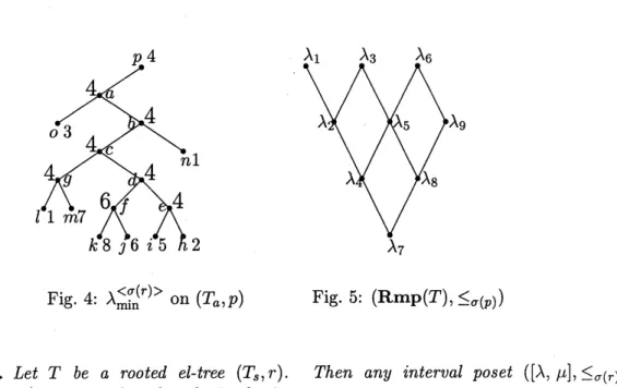
the $\sigma(r)$-version MPR-poset.The reconstruction $\lambda$ defined in Proposition 1 is particularly written as $\lambda_{\min}^{<\sigma(r)>}$. We here
show some examples for the least element $\lambda_{\min}^{<\sigma(r)}>$
.
Let the $\mathrm{e}1$-tree $T$ in Fig.1 be rooted at
$p$.
Then from the MPR-sets in Fig.$\mathrm{F}\mathrm{i}\mathrm{g}:\mathrm{M}\mathrm{P}\mathrm{R}_{\mathrm{S}}\mathrm{e}\mathrm{t}\mathrm{s}$ and Proposition 1, we obtain the least element
$\lambda_{\min}^{<\sigma(p)}>$ is shownin Fig.4, with the rooted
$\mathrm{e}1$-tree$T=(T_{a}, p)$
.
We alsosee
that $\lambda_{\min}^{<\sigma(p)}>$ is reallyequal to $\lambda_{7}$ in $\mathrm{R}\mathrm{m}\mathrm{p}(T)$ shown in Table 1, $\mathrm{i}.\mathrm{e}$, the least element of the
$\sigma(r)$-version MPR-poset
$(\mathrm{R}\mathrm{m}\mathrm{p}(\tau), \leq_{\sigma(p)})$ shown in Fig.5.
We see from Fig.5 that there is not necessarily the greatest element in a $\sigma(r)$-version
MPR-poset, that is, a$\sigma(r)$-version MPR-poset is not necessarilya complete distributivelattice, and so
we here examine the lattice-theoretic properties on intervals of any $\sigma(r)$-version MPR-poset.
For any $\lambda,$
$\mu$ which are comparable elements in a REC-poset, it is easily shown that the
interval subposet $([\lambda, \mu], \leq_{\sigma(r)})$ of the REC-poset has the greatest element $\mu$ and the infimum of
any nonempty subset of$[\lambda, \mu]$
.
Furthermore, when $\Lambda$ is of any two elements in$[\lambda, \mu],$ $\inf_{\sigma(r)}\Lambda$ is
to be themeet$(\wedge)$ of the twoelements, which isreally the minimum ofthe twoelements on
$\leq_{\sigma(r)}$,
and$\sup_{\sigma(r)}\Lambda$is thejoin$()$ of the twoelements, whichis really the maximum ofthe two elements
on $\leq_{\sigma(r)}$. Then we see easily that the distributive laws on the lattice-theoretic operations hold
in $([\lambda, \mu], \leq_{\sigma(r)})$
.
Thus we have that any interval poset $([\lambda, \mu], \leq_{\sigma(r)})$ in $(\mathrm{R}\mathrm{e}\mathrm{C}(\tau), \leq_{\sigma(r)})$ is acomplete distributive lattice.
By the similar way stated above, we obtain the following which is the third main theorem in
Fig. 4: $\lambda_{\min}^{<\sigma(r)}>$ on
$(T_{a},p)$ Fig. 5: $(\mathrm{R}\mathrm{m}\mathrm{p}(\tau), \leq_{\sigma(p)})$
Theorem 3. Let $T$ be a rooted $el$-tree $(T_{s}, r)$
.
Then any interval poset $([\lambda, \mu], \leq_{\sigma(r)})$ in$(\mathrm{R}\mathrm{m}\mathrm{p}(\tau), \leq_{\sigma(r)})$ is a complete $di_{S}t\dot{n}butive$ lattice.
We finally give
some
remarks. It is easily shown that the results in this paper are naturallygeneralized to the multi-character
case
for an $\mathrm{e}1$-tree. One alsosee
easily that an MPR-lattice isnot always a complemented lattice. In a later paper, we investigate in detail the order-theoretic
structures ofa$\sigma(r)$-version MPR-poset. We particularly give
some
characterizations of maximalelements in that poset and then
a
necessary and sufficient condition for that poset to have thegreatest element, i.e., to be acomplete distributive lattice.
References
[1] M. Blum, R. W. Floyd, V. Pratt, R. L. Rivest, and R. E. Tarjan, Time bounds forselection, JCSS 7 (1973)
448-461.
[2] J. M. Farris, Methods for computing Wagner trees, Systematic Zoology 19 (1970)83-92.
[3] M. Hanazawa, H. Narushima and N. Minaka, Generating most parsimonious reconstructions on a tree: a
generalization of the$\mathrm{F}\mathrm{a}\mathrm{r}\mathrm{r}\mathrm{i}_{\mathrm{S}}-\mathrm{S}_{\mathrm{W}}\mathrm{o}\mathrm{f}\mathrm{f}\mathrm{o}\mathrm{r}\mathrm{d}_{- \mathrm{M}\mathrm{a}}\mathrm{d}\mathrm{d}\mathrm{i}_{\mathrm{S}0\mathrm{n}}$method, Discrete Applied Mathematics 56 (1995) 245-265.
[4] N. Minaka, Parsimony, phylogeny and discrete mathematics: combinatorial problems in phylogenetic sys, tematics (in Japanese: with English summary), Natural History Research, Chiba Prefectural Museum and Institute, Vol.2No.2 (1993)83-98.
[5] N. Minaka, Algebraic properties ofthemost parsimonious reconstructions ofthehypothetical ancestorson a giventree,Forma 8 (1993) 277-296.
[6] H.Narushima and M.Hanazawa, Amoreefficientalgorithm for MPR problems in phylogeny, DiscreteApplied
Mathematics 80 (1997)231-238.
[7] H. Narushima and N. Misheva, On a role of the MPR-poset of most-parsimonious reconstructions in
phy-logenetic analysis –A combinatorial optimization problem in phylogeny-, in: W. Y. C. Chen, D. Z. Du, D. F. Hsu, H. Y. Hap (Eds.), Proc. The International Symposiumon Combinatoircs and$\mathrm{A}.\mathrm{p}\mathrm{p}\mathrm{l}\mathrm{i}_{\mathrm{C}}\mathrm{a}\mathrm{t}\mathrm{i}_{\mathrm{o}\mathrm{n}}\mathrm{S}$ 28-30,
June, 1996, Tianjin, P.R.China, pp.
30.6-313.
[8] H. Narushima, On globally optimal reconstructions of phylogenetic trees(inJapanese: with apartinEnglish),
RIMS Koukyuuroku992 $‘(\mathrm{C}_{\mathrm{o}\mathrm{m}\mathrm{p}\mathrm{u}\mathrm{t}}\mathrm{a}\mathrm{t}\mathrm{i}\mathrm{o}\mathrm{n}$ Theoryand Its applications” (Kyoto Univ., May, 1997), pp. 5-11.
[9] H. Narushima and N. Misheva, On characteristics of ancestral character-state reconstructions under the ac-celerated transformation optimization, preprint.
[10] H. Narushima, On extremal properties of ACCTRAN reconstructions in phylogeny, preprint.
[11] D. L. Swofford and W. P. Maddison, Reconstructing ancestral character states under Wagner parsimony, Mathematical Biosciences 87 (1987) 199-229.
[12] D. L. Swofford, W. P. Maddison, Parsimony,character-state reconstructions, and evolutionary inferences, in: R. L. Mayden (Ed.), Systematics, Historical Ecology, and NorthAmerican Reshwater Fishes,Stanford Univ.