T it le: N u m eri ca l St u d y of H el ica l Pi p e F lo w Sep tem b er, 2 0 1 7 A n u p K u m er D at ta
Numerical Study of Helical Pipe Flow
Ph.D Thesis
September, 2017
Anup Kumer Datta
The Graduate School of Natural Science and Technology (Doctor Course)
OKAYAMA UNIVERSITY, JAPAN
Numerical Study of Helical Pipe Flow
A thesis
Submitted in partial fulfillment of the requirements for the degree of
Doctor of Philosophy
by
Anup Kumer Datta
Under the supervision of
Professor Shinichiro YANASE
The Graduate School of Natural Science and Technology (Doctor Course)
Okayama University, Japan September, 2017
Dedication
This dissertation is dedicated to my late father who shaped part of my vision and taught me the good things that really matter in life
Anup Kumer Datta
September, 2017
i
Contents
Abstract……… 1
Acknowledgement……… 3
List of Figures……….. 4
List of Tables……… 10
Nomenclature………... 11
Dissertation contents……… 13
Chapter 1 Introduction………. 16
1.1 Definition of some useful parameters……….. 17
1.2 Flow in curved pipes………. 19
1.3 Flow in helical pipes………. 21
1.3.1 Non-orthogonal coordinate system………. 23
1.3.2 Orthogonal coordinate system………. 24
1.4 Flow pattern through curved and helical pipes………. 28
1.5 Influence of pitch on the flow pattern……… 32
1.6 Stability of the flow in a helical pipe……… 33
1.7 Pressure drop and friction factor……….. 36
1.8 Heat transfer of flow through curved and helical pipes…… 39
Chapter 2 Mathematical formulation……….. 51
2.1 Mathematical formulation and governing equations……… 51
2.2 Turbulence models……… 54
2.2.1 RNG 𝑘 − 𝜀 model………. 55
2.2.2 Lien-cubic 𝑘 − 𝜀 model……… 56
2.2.3 Launder-Sharma 𝑘 − 𝜀 model………... 57
2.3 Boundary conditions………. 58
Chapter 3 Numerical methods………. 59
3.1 Numerical methods………... 59
3.2 Finite volume discretization………. 59
3.2.1 Discretization of the solution domain……… 60
ii
3.3 Discretization of the transport equation……… 62
3.3.1 Discretization of spatial terms……… 64
3.3.1.1 Convection term……….. 65
3.3.1.2 Convection differencing scheme………….. 66
3.3.1.3 Diffusion term……….. 68
3.3.1.4 Source term……….. 69
3.4 Temporal discretization ……… 70
3.5 Solution techniques………... 73
3.6 Discretization procedure for the Navier-Stokes system……. 76
3.6.1 Derivation of the pressure equation……… 78
3.6.2 Pressure-velocity coupling………. 79
3.6.2.1 The PISO algorithm for transient flows…… 79
3.6.2.2 The SIMPLE algorithm……… 80
3.6.3 Solution procedure for the Navier Stokes equation… 82 Chapter 4 Laminar flow through a helical pipe with circular cross section………... 85
4.1 Objectives and scope of this chapter………. 84
4.2 Results………... 86
4.2.1 Two dimensional steady state and the definition of Re and Dn………. 86 4.2.2 Dean number calculated in the present study……… 89
4.2.3 Secondary flow for 𝛿 = 0.4……….. 90
4.2.4 Axial flow for 𝛿 = 0.4………... 92
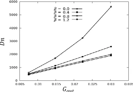
4.2.5 Flux through the pipe………. 94
4.3 Unsteady solutions……… 95
4.3.1 Method to obtain the critical Reynolds number……. 95
4.3.2 Critical Reynolds number for various 𝛽……… 97
4.3.3 Time evolution of the equi-surface of the axial flow velocity ………. 99
4.4 Discussion and conclusion……… 105
Chapter 5 Effect of torsion on the friction factor of helical pipe flow….. 107
iii
5.1 Objectives and scope of this chapter……….. 107
5.2 Results……….. 108
5.2.1 Comparison with the experimental data for Type -1 110 5.3 Axial flow distribution for Type -1……….. 114
5.4 Friction factor over a wide range of 𝛽……….. 116
5.4.1 Friction factor for Type -1 (𝛿 = 0.1)……….. 116
5.4.2 Friction factor for Type -2 (𝛿 = 0.05)………. 119
5.5 Discussion and conclusion……… 122
Chapter 6 Thermal flow through a helical pipe with circular cross section………... 124
6.1 Objectives and scope of this chapter………. 125
6.2 Results………... 125
7.2.1 Nusselt number……….. 126
6.3 Torsion effect on the Nusselt number……… 127
6.4 Torsion effect on the secondary flow and temperature field.. 129
6.5 Local Nusselt number……… 133
6.6 Discussion and conclusion……… 134
Chapter 7 Turbulent flow through a helical pipe with circular cross section………... 136 7.1 Objectives and scope of this chapter………. 136
7.2 Results………... 138
7.3 Results of the case for 𝛽 = 0.02……… 140
7.4 Results of the case for 𝛽 = 0.45……… 148
7.5 Discussion and conclusion……… 154
Chapter 8 General conclusions……… 158
References ………
1621
Abstract
Flows and heat transfer in helical pipes have attracted considerable attention not only because of their ample applications in chemical, mechanical, civil, nuclear and biomechanical engineering but also their physical interest of secondary flow patterns and soon. In this dissertation, three dimension (3D) direct numerical simulations (DNS) of viscous incompressible isothermal (without heat transfer) and thermal (with heat transfer) laminar and turbulent fluid flows through a helical pipe with circular cross section are presented, where the wall of a helical pipe is heated for thermal case. Note that the case of turbulent flow through a helical pipe, we also used three different turbulent models based on the Reynold averaged Navier-Stokes equation (RANS). Numerical calculation were carried out over a wide range of Dean number, Dn, curvature, 𝛿, torsion parameter, 𝛽, the Prandtl number, Pr, and the Reynolds number, Re, for both the laminar and turbulent flow cases.
OpenFOAM was used as a tool for the numerical approach. To generate a suitable mesh in the flow domain, an appropriate mesh system with 3D orthogonal helical coordinates was successfully created to conduct accurate DNSs and turbulence models of helical pipe flow using an FVM-based open-source computational fluid dynamics package (OpenFOAM).
First, the laminar flow in a helical pipe with circular cross section was investigated. The instability of the steady solutions of the helical pipe flow was studied instead of the linear stability analysis. We found the neutral curve of the critical Reynolds numbers of the laminar to turbulent transition by observing unsteady behaviors of the solution. The present results of the critical Reynolds number nearly agree with the two-dimensional (2D) linear stability analysis (Yamamoto et al. (1998)) except for the lowest critical Reynolds number region, where the present study gave the critical Reynolds numbers much less than those by the 2D linear stability analysis and showed explosive 3D instability occurred slightly in the marginal instability state. It is interesting that we found a close relationship between the disturbances of unsteady solutions (such as nearly 2D state, nonlocal 3D modification, highly nonlinear behaviours, continuous nonperiodic oscilation), and the vortical structure of steady solutions in helical pipe flow.
2
Then, the effect of torsion on the friction factor of helical pipe flow was investigated. Well- developed axially invariant regions were obtained where the friction factors were calculated, and good agreement with the experimental data was obtained. It was found that the friction factor sharply increases as 𝛽 increases from zero, then decreases after taking a maximum, and finally slowly approaches that of a straight pipe when 𝛽 tends to infinity. It is interesting that a peak of the friction factor exists in the region 0.2 ≤ 𝛽 ≤ 0.3 for all the Reynolds numbers and curvatures studied in the present study, which manifests the importance of the torsion parameter in helical pipe flow.
Next, laminar forced convective heat transfer in a helical pipe with circular cross section subjected to wall heating was investigated comparing with the experimental data. In 3D steady calculations, we found the appearance of fully-developed axially invariant flow regions, where the averaged Nusselt number (averaged over the peripheral of the pipe cross section) were calculated, being in good agreement with the experimental data. Because of the effect of torsion on the heat transfer characteristics, the averaged Nusselt number exhibits repetition of decrease and increases as torsion increases from zero for all Reynolds numbers.
It was found that there exists two maximums and two minimums of the averaged Nusselt number. It is interesting that the global minimum of the Nusselt number occurs at 𝛽 ≅ 0.1 and the global maximum at 𝛽 ≅ 0.55.
Finally, turbulent flow through helical pipes with circular cross section was numerically investigated by use of three different turbulence models comparing with the experimental data. We numerically obtained the secondary flow, the axial flow and the intensity of the turbulent kinetic energy by use of three turbulence models. We found that the change to fully developed turbulence is identified by comparing experimental data with the results of numerical simulations using turbulence models. We found that RNG 𝑘 − 𝜀 turbulence model can predict excellently the fully developed turbulent flow with comparison to the experimental data. It was found that the momentum transfer due to turbulence dominates the secondary flow pattern of the turbulent helical pipe flow. It is interesting that torsion effect is more remarkable for turbulent flows than laminar flows.
3
Acknowledgement
First of all, I would like to express my heartiest gratitude and appreciation to Professor Shinichiro YANASE, Department of Mechanical Engineering, Okayama University, Japan, who accepted me as one of his Ph.D students and under whose guidance the work was accomplished. His enthusiastic guidance and vigilant supervision made it easy to successfully complete the work on time. My sincere thanks to him for his wonderful advice and valuable suggestions in every stage of my study from project selection to the dissertation writing. I am deeply indebted to him. I would also like to thank him for his earnest feelings and necessary helps concerning my personal affairs during the whole period of my study in Japan.
I express my deep regards and sincere thanks to Professor Akihiko HORIBE and Professor Eiji TOMITA, Department of Mechanical Engineering, Okayama University, Japan. Sincere appreciation is extended to Emirates Professor Kyoji YAMAMMOTO and Dr. Toshinori KOUCHI, Associate Professor of the same department and Dr. Yasutaka Hayamizu, Associate Professor, National Institute of Technology, Yonago College, Tottori, Japan for their valuable advice and suggestion, especially during the study of numerical simulation. I take the opportunity to thanks all the research students of this laboratory for their helps and friendly attitude during the whole period of study.
I am grateful to the Japanese Ministry of Education, Culture, Sports, Science and Technology for offering me the financial support through MEXT scholarship to conduct this study. My special thanks go for this institution.
Finally, I would also like to express my dearest appreciation and indebtedness to my wife Swapna Mondal for her constant cooperation and special sacrifice in letting me put most of my time in Lab during my study. Last, but not least, my profound debts to my family members, relatives and friends are also unlimited for their continuous inspiration and moral support in pursuing this work.
4
List of figures
1.1 Helical pipe with circular cross section………. 22
1.2 Helical coordinate system used by Wang (1981)……….. 24
1.3 Helical coordinate system used by Germano……… 25
2.1 (a) Helical pipe with circular cross section, (b) coordinate system………. 52
3.1 Control volume (H. Jasak (1996))………. 61
3.2 Face interpolation……….. 66
3.3 Vector d and S on a non-orthogonal mesh.………... 68
3.4 Non-orthogonality treatment in the “orthogonal correction” approach……… 69
4.1 Pressure p versus z for 𝛿 = 0.4 and Dn = 1000………. 88
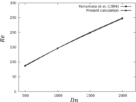
4.2 Dn of the helical pipe flows for 𝛿 = 0.4, where Dn is calculated by Eq. (1.6) with 𝐺𝑖𝑛𝑡 used for G………... 89 4.3 Re versus Dn for 𝛽 = 0.8 and 𝛿 = 0.4 ………... 90
4.4 Vector plots of the secondary flow and contours of the Q-value for Dn = 1000 and 𝛿 = 0.4. The present DNS results are on the cross section in the fully developed 2D region, where an outer wall is on the right-hand side of each figure. The thick lines denote the contour of the Q-value, where Q = 0.75 for 𝛽 = 0.0 and Q = 1.5 for other cases of 𝛽. Figure 4.4(a) is for 𝛽 = 0.0 at z = 0.008 m, (b) 𝛽 = 0.4 at z = 0.19 m, (c) 𝛽 =0.8 at z = 0.36 m and (g) 𝛽 =1.2 at z = 0.29 m. Figure 4.4 (d), (e), (f) and (g) are the corresponding results of the 2D spectral study (Yamamoto et al. (1994))……….. 91
4.5 Contours of the axial velocity for Dn = 1000 and 𝛿 = 0.4. The present DNS results are the axial velocity on a cross section in the fully developed 2D region. Figure 4.5(a) is for 𝛽 = 0.0 at z = 0.008 m, (b) 𝛽 = 0.4 at z = 0.19 m (c) 𝛽 =0.8 at z = 0.36 m and (g) 𝛽 =1.2 at z = 0.29 m. Figures (d), (e) (f) and (g) are the corresponding results of the 2D study (Yamamoto et al. (1994)). The increment of the velocity is 20. ………... 93
5
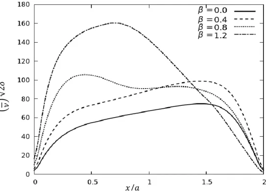
4.6 The distribution of the axial velocity for Dn = 1000 and 𝛿 = 0.4 on the center
line (y = 0)……….. 94
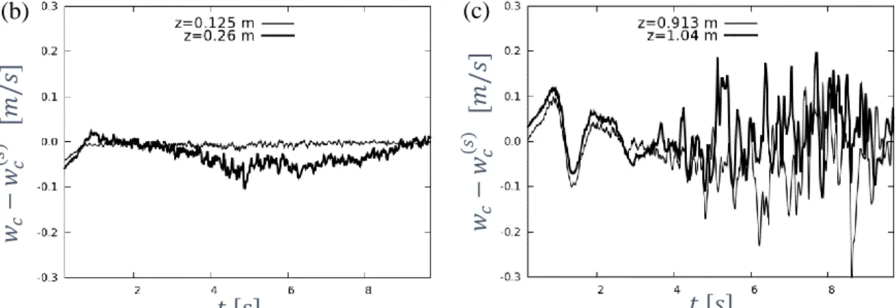
4.7 Flux ratio Q/Qs for for Dn = 1000 and 𝛿 = 0.4……… 95 4.8 Time-evolution of the deviation of the axial velocity from the steady solution
at various valus of z on the center line for 𝛽 = 0.6 and 𝛿 = 0.1. Figure 4.8(a) is for Re = 1096 and (b), (c) for Re = 1100………... 96 4.9 The critical Reynolds number in the 𝑅𝑒-𝛽 plane for 𝛿 = 0.1. The symbol ●
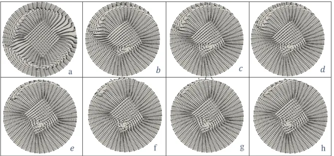
denotes the present DNS results. The results of the 2D linear stability by Yamamoto et al. (1998) are shown with the symbol ▽, and the experimental data by Hayamizu et al. (2008) with the symbol ○………. 98 4.10 Equi-surface of the constant velocity of w for Re = 1090, 𝛽 = 0.6 and 𝛿 =0.1
in the region z = 0.43 m-0.90 m. Figure 7(a) is the pipe wall, (b) at t = 0.5 s, (c) t = 0.8 s, (d) t = 1.0 s, (e) t = 1.5 s, (f) t = 1.8 s, (g) t = 3.0 s and (h) t = 5.0
s………. 100
4.11 Vector plots of the secondary flow for Re =1090, and 𝛽 = 0.6 at z = 0.39, where an outer wall is on the right-hand side of each figure.. Figure 4.11(a) is for 𝑡 = 0.2s, (b) 𝑡 = 1.2s, (c) 𝑡 = 1.8s, (d) 𝑡 = 2.1s, (e) 𝑡 = 5s, (f) 𝑡 = 7.2s, (g) 𝑡
= 8s, and (g) (c) 𝑡 = 9.35s………... 101 4.12 Contours of the axial flow for Re =1090, and 𝛽 = 0.6 at z = 0.39. 𝑊𝑚𝑎𝑥 is
maximum position of the axial velocity., where an outer wall is on the right- hand side of each figure.. Figure 4.12(a) is for 𝑡 = 0.2s, (b) 𝑡 = 1.2s, (c) 𝑡 = 1.8s, (d) 𝑡 = 2.1s, (e) 𝑡 = 5s, (f) 𝑡 = 7.2s, (g) 𝑡 = 8s, and (g) (c) 𝑡 = 9.35s……... 102 4.13 Vector plots of the secondary flow for Re =1090, and 𝛽 = 0.6 at z = 0.774,
where an outer wall is on the right-hand side of each figure.. Figure 4.13(a) is for 𝑡 = 0.2s, (b) 𝑡 = 1.2s, (c) 𝑡 = 1.8s, (d) 𝑡 = 2.1s, (e) 𝑡 = 5s, (f) 𝑡 = 7.2s, (g) 𝑡
= 8s, and (g) (c) 𝑡 = 9.35s………... 102 4.14 Contours of the axial flow for Re =1090, and 𝛽 = 0.6 at z = 0.774. 𝑊𝑚𝑎𝑥 is
maximum and 𝑊𝑚𝑖𝑛 is minimum position of the axial velocity., where an outer wall is on the right-hand side of each figure.. Figure 4.14(a) is for 𝑡 =
6
0.2s, (b) 𝑡 = 1.2s, (c) 𝑡 = 1.8s, (d) 𝑡 = 2.1s, (e) 𝑡 = 5s, (f) 𝑡 = 7.2s, (g) 𝑡 = 8s,
and (g) (c) 𝑡 = 9.35s………... 103
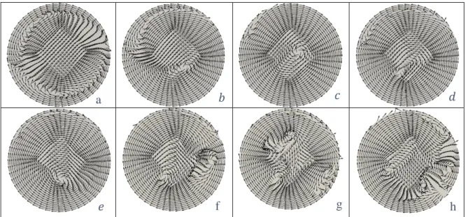
4.15 Equi-surface of the constant velocity of w for Re = 110, 𝛽 = 1.6 and 𝛿 =0.1 in the region z = 0.42 m-0.66 m. Figure 8(a) is the pipe wall, (b) at t = 2.0 s, (c) t = 5.0 s, (d) t = 6.6 s, (e) t = 6.8 s, (f) t = 7.0 s and (g) t = 7.2 s……… 104
4.16 Equi-Q value surface for Re = 110, 𝛽 = 1.6 and 𝛿 =0.1 in the region z = 0.42 m-0.66 m. Figure 9 (a) is the pipe wall, (b) at t = 2.0 s, (c) 5.0 s, (d) 6.6 s, (e) 6.8 s, (f) 7.0 s and (g) 7.2 s……….. 105
5.1 Contours of the axial velocity for Re = 145 and 𝛿 = 0.4. The present DNS results are the axial velocity on a cross section in the fully developed region. (a) 𝛽 =0.8 at z = 0.36 m. (b) corresponding results of the spectral study Yamamoto et al. (1994). The increment of the contours is 20 and the outer wall is on the right side………... 110
5.2 Friction factor of the helical pipe for β = 0.45 and 𝛿 = 0.1. ……….. 111
5.3 Friction factor of the helical pipe flow at 𝛿 = 0.1 for β = 0.91………... 112
5.4 Friction factor of the helical pipe flow at 𝛿 = 0.1 for β = 1.17……… 113
5.5 Friction factor of the helical pipe flow at 𝛿 = 0.1 for β = 1.57……… 113
5.6 Friction factor of the helical pipe flow at 𝛿 = 0.1 for β = 1.70……… 114
5.7 Distribution of the axial velocity for 0.45 ≤ 𝛽 ≤ 1.70 and Re = 1000 at 𝛿 = 0.1 on the center line (y = 0)………. 115 5.8 Distribution of pressure for 0.45 ≤ 𝛽 ≤ 1.70 and Re = 1000 at 𝛿 = 0.1 on the center line (y = 0)……….. 116 5.9 Friction factor of the helical pipe for Re = 80 at 𝛿 = 0.1……… 117
5.10 Friction factor of the helical pipe for Re = 300 at 𝛿 = 0.1……….. 117
5.11 Friction factor of the helical pipe for Re = 1000 at 𝛿 = 0.1……… 118
5.12 Friction factor of the helical pipe for Re = 80 at 𝛿 = 0.05………... 119
5.13 Friction factor of the helical pipe for Re = 300 at 𝛿 = 0.05………. 120
5.14 Friction factor of the helical pipe for Re = 1000 at 𝛿 = 0.05………... 120
7
6.1 The Nusselt number for 𝛽 = 0.0012 and 𝛿 = 0.018. The symbols ● and ▲ represents the present DNS results for Pr = 8.5 and 7.5, respectively, and the experimental data by Shatat (2010) with the symbol ■ forPr = 8.5……… 127 6.2 The Nusselt number for 𝛿 = 0.018 at Pr = 4.02. The symbol ▼ represents the
Nu for 𝛽 = 0.1, ○ for 𝛽 = 0.3, ▲ for 𝛽 = 0.45 and □ for 𝛽 = 0.8………. 128 6.3 The Nusselt number as a function of 𝛽 for 𝛿 = 0.018 at Pr = 4.02. The line
of ○ for 𝑅𝑒 = 1047, □ for Re = 1633 and ▲ for 𝑅𝑒 = 2600……….. 129 6.4 Vector plots of the secondary flow and contours of the Q-value for Re = 1047,
𝛿 = 0.018 and Pr = 4.02, where an outer wall is on the right-hand side of each figure. The thick lines denote the contour of the Q-value, where Q = 1.0 for all figures. Figure 6.4 (a) is for 𝛽 = 0.002 at z = 0.16 m, (b) 𝛽 = 0.1 at z = 5.95 m and (c) 𝛽 = 0.55 at z = 2.01 m………. 131 6.5 2D stream lines of the secondary flow for Re = 1047, 𝛿 = 0.018 and Pr =
4.02, where an outer wall is on the right-hand side of each figure. Figure 6.5 (a) is for 𝛽 = 0.002 at z = 0.16, m (b) 𝛽 = 0.1 at z = 5.95 m and (c) 𝛽 = 0.55 at
z = 2.01 m………... 131
6.6 Contours of the temperature field for Re = 1047, 𝛿 = 0.018 and Pr = 4.02, where the outer wall is on the right-hand side of each figure. Figure 6.6 (a) is for 𝛽 = 0.002 at z = 0.16 m, (b) 𝛽 = 0.1 at z = 5.95 m and (c) 𝛽 = 0.55 at z = 2.01 m. The increment of the temperature is -10 for 𝛽 =0.002 and 0.1 and -20
for 𝛽 = 0.55……….... 132
6.7 Local Nusselt number distribution for Re = 1047, 𝛿 = 0.018 and Pr = 4.02.
The solid is for 𝛽 = 0.002 at z = 0.16 m, a dashed line for 𝛽 = 0.1 at z = 5.95 m and a dotted line for 𝛽 = 0.55 at z = 2.01 m. ……… 133 7.1 A view of the 3.2 pitch helical pipe showing the three-pitch downstream cross
section for 𝛽 = 0.02 and 𝛿 = 0.1………... 138 7.2 Axial flow distribution on the x-axis for 𝛽 = 0.02 and 𝛿 = 0.1……….. 139 7.3 Axial velocity distribution on the x-axis for 𝛽 = 0.02 at 𝛿 = 0.1. The outer
wall is on the right-hand side……….. 141
8
7.4 Axial velocity distribution on the y-axis for 𝛽 = 0.02 at 𝛿 = 0.1. The upper wall is on the right-hand side……….. 142 7.5 Vector plots of the secondary flow for β = 0.02 and 𝛿 = 0.1. Two figures on
the left-hand side are the results of numerical simulations and one on the right- hand side is the experimental result. (a) is for Re = 12140 and (b) for Re = 20850. The outer wall is on the right-hand side……….. 143 7.6 Fig. 7.6. Numerical result of vector plots of the secondary flow for β = 0.02
and 𝛿 = 0.1 at Re = 200……… 144
7.7 Contours of the axial velocity for β = 0.02 and 𝛿 = 0.1. Two figures on the left-hand side are the results of numerical simulations and one on the right- hand side is the experimental result. (a) is for Re = 12140 and (b) for Re =
20850………. 146
7.8 Turbulent intensity, (2𝑘)1 2⁄ /〈𝑤〉 for β = 0.02 and 𝛿 = 0.1 at Re = 12140 and 20850, where 𝑘 is the intensity of turbulent kinetic energy and 〈𝑤〉 the mean axial velocity. Two figures on the left-hand side are the results of numerical simulations and one on the right-hand side is the experimental result. (a) is for Re = 12140 and (b) for Re = 20850………. 147 7.9 Axial velocity distribution on the x-axis for 𝛽 = 0.45 at 𝛿 = 0.1. The outer
wall is on the right-hand side……….. 149 7.10 Axial velocity distribution on the y-axis for 𝛽 = 0.45 at 𝛿 = 0.1. The upper
wall is on the right-hand side……….. 150 7.11 Contours of the axial velocity for β = 0.45 and 𝛿 = 0.1. Two figures on the
left-hand side are the results of numerical simulations and one on the right- hand side is the experimental result. (a) is for Re = 9340 and (b) for Re =
19910………. 152
7.12 Turbulence intensity,(2𝑘)1 2⁄ /〈𝑤〉, for β = 0.45 and 𝛿 = 0.1 at Re = 9340 and 19910, where k is the intensity of turbulent kinetic energy and 〈𝑤〉 the mean axial velocity. Two figures on the left-hand side are the results of numerical
9
simulations and one on the right-hand side is the experimental result. (a) is for Re = 9340 and (b) for Re = 19910………...
153 7.13 Friction factor of the helical pipe for β = 0.45 and 𝛿 = 0.1 ………. 154 7.14 Equi-Q value surface for β = 0.02 and 𝛿 = 0.1. (a) shows the pipe wall, (b)
the case for Re = 200, where Q = 0.5 and (c) the case for Re = 20850, where
Q = 70……… 155
7.15 Equi-Q- value surface for β = 0.45 and 𝛿 = 0.1. (a) shows the pipe wall, (b) the case for Re = 200, where Q = 0.5 and (c) the case for Re = 19910, where
Q = 70……… 156
10
List of Tables
1.1 Curvature and torsion data for helical pipes……….. 22 4.1 Grid sensitivity analysis for steady solutions for Dn = 1000 and 𝛿 = 0.4 at
𝛽 = 0.8………..
87 4.2 Grid sensitivity analysis for unsteady calculations. The symbol ○ indicates
the stable and □ the unstable……….
97 4.3 The critical Reynolds number. 𝑅𝑒𝑐1 is the Reynolds number of the
marginally stable state and 𝑅𝑒𝑐2 is that of the marginally unstable state……..
99
5.1 Characteristic lengths of the helical pipes 108
5.2 Grid sensitivity analysis for Re = 200 and 𝛿 = 0.1 at 𝛽 = 1.2………... 109 5.3 Friction factors for three Reynolds numbers at 𝛿 = 0.1 and 0.05………... 121 6.1 Grid sensitivity analysis for Re = 1633 and 𝛿 = 0.018 at 𝛽 = 0.0012……… 126 7.1 Grid sensitivity analysis for Re = 5320 for 𝛽 = 0.02 at 𝛿 = 0.1. ……….. 139
11
Nomenclature
𝑑𝑝 diameter of the pipe H pitch of the helical pipe
t unit tangential vector n unit normal vector b unit binormal vector
R distance of the center line from the axis of the whole system Pr Prandtl number
k Turbulent kinetic energy 𝑇𝑤 Wall temperature
𝑅ℎ Radius of curvature P Pressure
𝑇𝑏 bulk temperature 𝐷𝑛 Dean Number
Re Reynolds number Nu Nusselt number 𝑞𝑤 rate of heat flux
u velocity component in the x-direction v velocity component in the y-direction w velocity component in the z-direction
〈𝑤〉 Ensemble-average axial velocity.
x horizontal axis y vertical axis
z axis in the direction of the main flow a Radius of the pipe
12
Greek letters 𝛿 curvature
𝛽 torsion parameter 𝛼 thermal diffusivity 𝜇 viscosity
𝜏 torsion
𝜐 kinematic viscosity 𝜌 density
13
Dissertation contents
This dissertation consists of the following papers and conference proceedings
Papers
1. Anup Kumer Datta, Yasutaka Hayamizu, Toshinori Kouchi, Yasunori Nagata, Kyoji Yamamoto and Shinichiro Yanase, (2017). Numerical study of turbulent helical pipe flow comparison to the experimental results
,
ASME Journal of Fluid Engineering, Vol. 139(9), pp. 091204(1-13).2. Anup Kumer Datta, Shinichiro Yanase, Yasutaka Hayamizu, Toshinori Kouchi, Yasunori Nagata and Kyoji Yamamoto, (2017). Effect of torsion on the friction factor of helical pipe flow
,
Journal of Physical Society of Japan, Vol. 86, pp. 064403(1- 7).3. Anup Kumer Datta, Shinichiro Yanase, Toshinori Kouchi, and Mohammed M.E.
Shatat, (2017). Laminar forced convective heat transfer in helical pipe flow
,
International Journal of Thermal sciences, Vol. 120, pp. 41-49.
Conference Proceedings and Poster
1. Anup Kumer Datta, Yasutaka Hayamizu, Yasunori Nagata, Toshinori Kouchi, Kyoji Yamamoto and Shinichiro Yanase (2015). Numerical study of transition in helical pipe flow. Proceedings, branch meeting of the Japan Society of Fluid Mechanics, November 28-29, 2015, Tottori University, Japan.
2. Anup Kumer Datta, Yasutaka Hayamizu, Toshinori Kouchi, Yasunori Nagata, Kyoji Yamamoto and Shinichiro Yanase (2016). Numerical and experimental study of turbulent helical pipe flow. Proceedings, International symposium on near-wall flows and turbulence, June 20-22, 2016, Kyoto University, Japan.
3. Anup Kumer Datta, Yasutaka Hayamizu, Toshinori Kouchi, Yasunori Nagata, Kyoji Yamamoto and Shinichiro Yanase (2016). Numerical and experimental study of
14
turbulent helical pipe flow. Poster, International symposium on near-wall flows and turbulence, June 20-22, 2016, Kyoto University, Japan.
4. Anup Kumer Datta (2016). Numerical study laminar and turbulent helical pipe flows.
Poster, International student Symposium on power and mechanical engineering, August 30-31, 2016, Okayama University, Japan.
5. Anup Kumer Datta, Yasutaka Hayamizu, Toshinori Kouchi, Yasunori Nagata, Kyoji Yamamoto and Shinichiro Yanase (2016). Numerical simulation of turbulent helical pipe flows. Proceedings, Annual meeting of the Japan Society of Fluid Mechanics, September 26-28, Nagoya, Japan, Paper No. 20.
6. Anup Kumer Datta, Toshinori Kouchi, Yasutaka Hayamizu, Yasunori Nagata, Kyoji Yamamoto and Shinichiro Yanase (2016). Numerical study of the laminar-turbulent transition in helical pipe flows. Proceedings, the 30th Computational Fluid Dynamics Symposium, December 12-14Tokyo, Japan, Paper No. F07-4.
7. Anup Kumer Datta, Yasutaka Hayamizu, Toshinori Kouchi, Yasunori Nagata, Kyoji Yamamoto and Shinichiro Yanase (2017). Influence of torsion on the friction factor of helical pipe flow. Proceedings, 13th International Symposium on Experimental Computational Aerothermodynamics of Internal Flows, May 7-11, Okinawa, Japan, Paper No. ISAIF13-S-0015.
The present dissertation is designed as follows
In Chapter 1, an introduction regarding curved and helical pipe flow with circular cross section are presented from analytical, numerical and experimental. In chapter 2, the basic governing equation for laminar and turbulent flow, related to the problems considered hereafter, are shown. In chapter 3, the calculation techniques for solving the basic equations, presented in chapter 2, are discussed. In chapter 4, a specific problem of the laminar flow through a helical pipe with circular cross section is considered, where the flow characteristics are presented studying over a wide range of curvature, torsion, Dean number and Reynolds number based on spectral study, experimental data. The same problem has been extended for the effect of torsion on the friction factor of helical pipe flow in Chapter 5. In Chapter 6, we presented the turbulent flow characteristics through a helical pipe with circular cross section with best turbulent models. In Chapte7, forced
15
convective heat transfer in helical pipe flow is considered. Finally, general conclusions on all the problems dealt are given in Chapter 8.
16
Chapter 1 Introduction
Fluid flow in helical pipes occurs in many industrial systems such as heat exchangers, chemical reactors, well drilling, and stimulation operations in the petroleum industry, kidney dialysis devices, food and dairy processes, and blood oxygenators, among many others. The investigation of helical pipe flows motivated scientific engineering applications interest, but later their relevance to industrial applications such as chemical reactors and heat exchangers (Huang et al., 2001 and Rennie & Raghavan, 2006). The realization that physiological flows, such as that in the human aorta, involve both curvature and torsion (Caro et al., 1996), provided additional motivation to studying helical pipes (Zabielski & Mestel, 1998), they being the simplest of such geometries.
Due to the curvature of the helical pipes the flowing fluid experiences a centrifugal force, which depends on the local axial velocity of the fluid particle. As a result of the difference in the axial velocity between the particles owing in the center of the pipe cross section and those flowing near the pipe wall with the effect of the boundary layer, a secondary flow develops which forces the fluid from the core region of the pipe towards the outer wall of the pipe, and moves the fluid near the pipe outer wall to the pipe inner wall, and the flowing fluid; however, it also may increase the pressure gradient required to obtain a given mass flux, and thus may increase the amount of energy. Therefore, an extensive knowledge of the heat transfer and hydrodynamic characteristics of flow through a helical pipe is essential for a better design of heat exchangers and systems that contains such pipes. The first observations of the curvature effect on flow in coiled tubes were noted at the beginning of the 20th century. Grindley and Gibson (1908) noticed the curvature effect on flow in a coiled pipe while performing experiments on air viscosity. Since then, numerous experimental as well as theoretical and numerical studies including helical coils, which is a subset of curved pipes, have been reported on the flow and heat transfer through curved pipes. These studies have shown the effect of different parameters on the flow pattern, pressure drop and heat transfer characteristics through helical and curved passages. These parameters include the
17
geometrical values such as; effect of pitch and curvature of the pipe, and the physical properties of the flowing fluid, covering a wide range of flow fields, laminar or turbulent, steady or unsteady, and with or without heat transfer.
Before examining the existing literature on helical pipe flow, a basic summary of flow in curved pipes is first presented. This background provides a useful basis from which to understand both the solution techniques, and the results, found in the helical pipe literature.
The main objective of this chapter is to discuss the development of Dean vortices which play an important role in curved pipe flows and reduces the pair of Dean vortices which goes to the single vortex in helical pipe flows. The Dean vortices arising in curved pipe single-phase flows are known as an effective means for heat and mass transfer enhancement and without convective heat transfer in laminar-transition-turbulent region. On the other hand, the flow in a helical pipe shows similarity with a number of other centrifugally unstable system where no torsion has been induced in helical pipe flows. This review, therefore, focuses on the steady, time-dependent flow behavior and transition to fully developed turbulent flow with forced convective heat transfer flow phenomena in helical pipe.
1.1 Definition of some useful parameters Dean number
The Dean number 𝜅 is defined as:
𝜅 = 2 (
𝑎𝑅
) (
2𝑎𝑤𝜈)
2 (1.1) where 𝑤 is the mean axial velocity in the pipe, a is the radius of the pipe, R is the radius of curvature and𝜈
is the viscosity while the original form of the Dean number was defined by Dean (1928) as:𝐾 = 2 (
𝑎𝑅) (
𝑎𝑤𝜈)
2= (
2𝑎𝜈32𝑤𝑅2),
(1.2) where w is defined as a constant having the dimensions of a velocity. If we take 𝑤 = 𝑤, then 𝐾 and 𝜅 are related by 𝜅 = (2𝐾)1 2⁄ . For fully developed flow, the axial pressure gradient is18
constant, say 𝑅1 𝜕𝑝𝜕𝑧 = −𝐺(G constant), in dimensional form. We can then define a non- dimensional constant, 𝐶 = 𝐺𝑎2⁄𝜈𝑤, and rewrite (1.2) as
𝐾 =
2𝑎3𝜈2𝑅
(
𝐺𝑎2𝜇𝐶
)
2.
(1.3)If, following Dean (1928), we specify w as the maximum velocity (𝑤𝑚𝑎𝑥) in a straight pipe of the same radius and with the same pressure gradient, then C = 4 and Eq. (1.3) becomes
𝐾 =
𝜈2𝑎2𝑅3(
𝐺𝑎4𝜇2)
2= 2 (
𝑅𝑎) (
4𝜇𝜈𝐺𝑎3)
2=
8𝜇𝐺22𝜈𝑎27𝑅 (1.4) Whereas if we simply set C =1, Eq. (1.3) becomes𝐾 =
2𝑎3𝜈2𝑅
(
𝐺𝑎𝜇2)
2.
(1.5) The various versions of the Dean number based on 𝑤, the mean axial velocity, are natural for the experimentalist because this quanity, being readily measured provided a more convenient characterization of the flow than the more difficult measurement of pressure gradient. For fully developed flow it is little different whether one uses a form of the Dean number based on G , i.e. Eq. (1.3), since C = constant for such a flow. For these flows most theoretical and numerical investigations, beginning with McConalogue &Srivastava (1968), have used the square root of (1.5) and denoted this by Dn𝐷𝑛 = √
2𝑎𝜈2𝑅3(
𝐺𝑎𝜇2) =
𝐺𝑎3√2𝑎 𝑅𝜈𝜇 ⁄= 4√
2𝑎𝑅 𝐺𝑎4𝜈𝜇2,
(1.6) which is related to the original Dean number, (1.4), by 𝐷 = 4√𝐾.Nusselt number
Convection is one of the basic mechanisms of heat transfer between a solid body and a fluid.
It can be quantified by the convective heat transfer coefficients. This coefficient is, in turn, determined by a quantity known as the Nusselt number, abbreviated as Nu. The Nusselt number is dependent on the geometry of the heat transfer system and on physical properties of the fluid. It is a dimensionless parameter which measures the enhancement of heat transfer from a surface which exists in a real situation. Typically, it is used to measure the
19
enhancement of heat transfer when convection takes place. One of the first quantities introduced about heat transfer is the convective heat transfer coefficient
ℎ = 𝑞𝑤 𝑇𝑤− 𝑇𝑏
where, 𝑞𝑤 = −𝑘𝜕𝑇𝜕𝑦, 𝑇𝑤 is the wall temperature, and 𝑇𝑏 is the bulk temperature of the fluid The Nusselt number is defined as
𝑁𝑢 =
ℎ𝑑𝑘 (1.7)
Where, h is the convection heat transfer coefficient, d the characteristic length, and k the thermal conductivity of the fluid. The Nusselt number can also be viewed as being a dimensionless temperature gradient at the surface. Nu > 0 means that heat transfer occurs from solid body to the fluid, whereas Nu < 0 indicates heat transfer in the opposite direction.
Prandtl number
The Prandtl number, Pr, is a dimensionless parameter which approximates the ratio of kinematic diffusivity to thermal diffusivity. It describes the effect of fluid thermo-physical properties on heat transfer and is combined traditionally with other dimensionless parameters for evaluating fluid-surface interfacial heat transfer coefficient. It is defined as
𝑃𝑟 =
𝛼𝜈 (1.8)where 𝜈 is the kinematic viscosity and 𝛼 is the thermal diffusivity. The Prandtl number shows the relative importance of heat conduction and viscosity of a fluid.
1.2 Flow in curved pipes
Secondary flow in curved pipes was first reported by Eustice (1910, 1911), in his experiments injecting ink into water flowing through a coiled pipe. The first theoretical treatment of the problem was given by Dean (Dean 1928), which used the toroidal coordinate system (𝑟′, α, θ). The non-dimensional Navier-Stokes equations are written in this coordinate system, and then simplified. First, the velocities are rescaled to make the centrifugal-force terms the same order of magnitude as the viscous and inertial terms, as it is the centrifugal force that drives
20
the secondary motion. Two parameters characterize the flow in curved pipes, the Dean number, Dn and the curvature, δ. They are defined:
𝛿 = 𝑎 𝑅⁄
𝑅𝑒 =𝑤 2𝑎𝜈 , 𝐷𝑛 = 𝑅𝑒√𝛿. (1.9) The Dean number is essential, which is modifying defined by the Reynolds number. The loose coiling assumption that the pipe has very small curvature, i.e. 𝛿 = 𝑎 𝑅⁄ ≪ 1 is applied by setting the δ terms to zero. The flow is also assumed to be fully developed, that is, independent of the axial position, which gives the final formulation of the equations as:
∇
12𝑤 −
𝐷𝑛2 𝜕𝑝𝜕𝑧0=
𝐷𝑛2𝑟(𝜓
𝛼𝑤
𝑟− 𝜓
𝑟𝑤
𝛼),
(1.10)2
𝐷𝑛
∇
14𝜓 +
1𝑟
(𝜓
𝑟 𝜕𝜕𝛼
− 𝜓
𝛼 𝜕𝜕𝑟
) ∇
12𝜓 = −2𝑤 (sin𝛼𝑤
𝑟+
cos𝛼𝑟
𝑤
𝛼),
(1.11) with the boundary conditions𝜓 = 𝜓𝑟 = 𝑤 = 0 at 𝑟 = 1, where
∇12 ≡ 𝜕2
𝜕𝑟2+1 𝑟
𝜕
𝜕𝑟+ 1 𝑟2
𝜕2
𝜕𝛼2.
For small Dean numbers the solution can be explained in a series expansion of powers of Dn.
𝑤 = ∑
∞𝑛=0𝐷𝑛
2𝑛𝑤
𝑛(𝑟, 𝛼), 𝜓 = 𝐷𝑛 ∑
∞𝑛=0𝐷𝑛
2𝑛𝜓
𝑛(𝑟, 𝛼),
(1.12) The primary flow, 𝑤0, is the Poiseuille flow, and the secondary term, 𝜓1, shows a symmetric pair of counter-rotating helical vortices. A centrifugal pressure gradient is formed, which drives slower-moving fluid near the wall inward. The faster moving fluid in the core is moved, which is the second-order correction to the axial velocity, 𝑤2. There are several consequences of the secondary flow formation; the flow rate is reduced from the equivalent Poiseuille flow, extremes of shear stress form at the inner and outer bends and the transition to turbulence is delayed.In consideration of their importance, flows in a curved pipe have been studied extensively in the literature for several decades. Most of the studies were focused on the Engineering applications, like the friction factor correlation (Ito, 1959; Manlapaz &Churchill, 1980;
Ramshankar &Sreenivassan, 1983; Liu et al. 1994) and heat transfer (Mori &Nakayama,
21
1967; Yao & Berger, 1978). In the last few decades, the emphasis has been shifted towards more fundamental studies of flow development (Hille et al., 1985; Bara et al., 1992), transition and bifurcation phenomena (Winters, 1987; Kao, 1992; Yanase et al., 1989, 2002).
Recent works in this area deal with laminar to turbulence transition and the oscillating behavior of the unsteady flows (Canton et al., 2015; Kuhnen et al. 2015, 2016).
1.3 Flow in helical pipes
A helical pipe is a three-dimensional object that can be described by the parametric equations:
𝑥 = 𝑅 cos𝜃, 𝑦 = 𝑅sin𝜃, 𝑧 = ℎ𝜃, 0 ≤ 𝜃 ≤ 2𝜋 (1.13) where R is the radius or amplitude of the helix and h is a constant parameter, such that the wavelength, or one pitch length, of the helical pipe equals 2πh. The radius of curvature of the helical pipe center line is 𝑅ℎ = 𝑅 + ℎ2⁄𝑅, the nondimensional curvature of the pipe 𝛿 = 𝜅𝑎 = 𝑎𝑅 (ℎ⁄ 2+ 𝑅2) , the nondimensional torsion 𝜏 = 𝑎ℎ (ℎ⁄ 2+ 𝑅2) and the torsion parameter is defined by 𝛽 = 𝜏 √2𝛿⁄ as introduced by Kao (1987). The length of the pipe center line for one turn is 2𝜋√𝑅ℎ𝑅 .
These expressions clearly show that the ratio of curvature to torsion is a constant, equal to 𝑅 ℎ⁄ , indeed Lancret’s theorem (Scofield 1995) states that this is a necessary and sufficient condition for a curve to be helical.
The equation of the helical centerline can be written as a vector 𝑅(𝑡)
𝑅(𝜃) = 𝑅cos𝜃 𝒊 + 𝑅sin𝜃 𝒋 + ℎ𝜃 𝒌 (1.14) Alternatively, this can be parameterized in terms of the arc-length s, which is given by
s = ∫ √(
0𝑡 𝑑𝜃𝑑𝑥)
2+ (
𝑑𝑦𝑑𝜃)
2+ (
𝑑𝜃𝑑𝑧)
2𝑑𝜃
(1.15) For a helical pipe, the arc length simply increases linearly with the parameter 𝜃, and evaluates tos = √𝑅2+ ℎ2 𝜃
22
The Frenet triad of tangent T, normal N and binormal B unit vectors of a curve R(s) are defined as:
𝑻 = 𝑑𝑅
𝑑𝑠, 𝑵 =1 𝜅
𝑑𝒕
𝑑𝑠, 𝑩 = 𝑻 × 𝑵
where 𝛿 = 𝜖 = 𝜅𝑎 is the curvature introduced so far. Figure 1 shows several different helical pipe geometries for varying parameter values, the properties of which are given in Table 1.1.
This figure indicates that one limit of a helical geometry is a straight pipe, and the other limit is a toroidal pipe.
Table 1.1: Curvature and torsion data for helical pipes shown in Figure 1.1
Figure 1.1: Helical pipe with circular cross section
Pipe 2a [mm] h [mm] R[mm] δ τ β n
a 50.5 0 252.5 0.1 0 0 0
b 50.5 22.41 250.5 0.1 0.009 0.02 3.2
c 50.5 65.46 18.3 0.1 0.36 0.8 3.2
d 50.5 45.47 8.47 0.1 0.54 1.2 3
23
1.3.1 Non-orthogonal coordinate system
In the theoretical perspectives of the helical pipe flows, Wang (1981) formulated the Navier- Stokes equations in a non-orthogonal helical coordinate system. This is shown in Figure 1.2, and the key points are as follows.
The first axis of the coordinate system is given by the vector equation of the centerline:
𝑅 = 𝑋(𝑠)𝒊 + 𝑌(𝑠)𝒋 + 𝑍(𝑠)𝒌 (1.16)
where s is the arc length along the axis, and i, j, k are the standard unit vectors in a Cartesian frame. A coordinate system (r, θ, s) can then be defined, such that a Cartesian vector x is given by:
𝑥 = 𝑅(𝑠)𝑇 + 𝑟cos𝜃 𝑵(𝑠) + 𝑟sin𝜃 𝑩(𝑠) (1.17) The definition of the pipe boundary follows naturally by setting 𝑟 = 𝐷 2⁄ , an additional parameter that is the internal radius of the pipe. That is:
𝑥 = 𝑅(𝑠)𝑇 + (𝐷 2)⁄ cos𝜃 𝑵(𝑠) + (𝐷 2)⁄ sin𝜃 𝑩(𝑠) (1.18) Taking the dot product of the incremental change of eqn (1.17) with itself gives:
𝑑𝑥. 𝑑𝑥 = (𝑑𝑟)2+ 𝑟2(𝑑𝜃)2+ [(1 − 𝜅𝑟 cos𝜃)2+ 𝜏2𝑟2](𝑑𝑠)2+ 2𝜏𝑟2𝑑𝑠𝑑𝜃 (1.19) non-orthogonality
It is the last term in Eq. (1.19) which highlights the non-orthogonal nature of this coordinate system. The physical consequence of this non-orthogonality is that the axial velocity w is not perpendicular to the (r, θ) plane. Wang’s analysis assumes that the pipe is long enough for end effects to be ignored, that is, the velocities are independent of s, or fully developed. In addition, both the curvature and torsion are assumed to be small, with the flow steady and laminar, for the Reynolds number of order unity.
For small curvature and torsion the axial flow w is dominant, and is found to be Poiseuille flow. This allows a series expansion of the form
𝑤 = 𝑼 ∑𝑛𝑖=0𝜖𝑖𝑤𝑖 (1.20) for the axial velocity, where U is a velocity scale proportional to the axial pressure gradient, and 𝜖 = 𝜅𝑎 ≪ 1, for pipe radius a. The secondary flow velocity is expanded in the following way, using u as an example:
𝑢 = 𝑼 ∑𝑛𝑖=1𝜖𝑖𝑢𝑖 (1.21)
24
The secondary flow is therefore order-1, with stream function 𝜓 defining the velocities as 𝑢1 =1𝜂𝜕𝜓𝜕𝜂, 𝑢2 = −𝜕𝜓𝜕𝜂 (1.22)
Figure 1.2: Helical coordinate system used by Wang where η is the normalised radial position, r/a. The stream function solution is:
𝜓
𝑅𝑒= sin𝜃288(𝜂7− 6𝜂5+ 9𝜂3− 4𝜂) −14(𝑅𝑒𝜆) (𝜂4− 2𝜂2+ 1) (1.23) Dean vortices Torsion rotation
The first term in Eq. (1.23) is the stream function for the Dean vortices; a pure curvature effect. The second term is a pure rotation, indicated by the lack of 𝜃 dependence, which arises due to the effect of torsion on the flow, where 𝜆 = 𝜏 𝜅⁄ and is a constant of order unity.
Wang found that for 𝜆 𝑅𝑒 ≥ 1 24⁄ ⁄ torsion dominates, causing a single recirculation cell in the secondary flow. It is important to note that this torsion effect is of first-order, which is the same order as curvature. This is because ψ is an O(𝜖) term, a first order term in this expansion, and 𝜆𝜖 = 𝜏𝑎
1.3.2 Orthogonal coordinate system
Germano showed that it is possible to construct an orthogonal coordinate system by replacing θ, from Wang’s system, with θ +𝜙(s)+𝜙0, in the plane normal to the axis (Germano 1982), as shown in Figure 1.3. The Cartesian vector x therefore becomes:
25
𝑥 = 𝑅(𝑠)𝑇 + 𝑟cos(𝜃 + 𝜙(𝑠) + 𝜙0) 𝑵(𝒔) + 𝑟sin(𝜃 + 𝜙(𝑠) + 𝜙0) 𝑩(𝑠) (1.24) where 𝜙(𝑠) = − ∫ 𝜏(𝑠𝑠𝑠 ′)𝑑𝑠′
0
with 𝜙0 and 𝑠0 taking arbitrary values. Again performing the dot product of the incremental change as before:
𝑑x. 𝑑x = (𝑑𝑟)2+ 𝑟2(𝑑𝜃)2+ [1 + 𝜅𝑟 sin (𝜃 + 𝜙]2(𝑑𝑠)2 (1.25) which shows that the system is now orthogonal. The key result reported in this
Figure 1.3: Helical coordinate system used by Germano
paper is that the torsion has only a second order effect on the flow, contrary to the findings of Wang (Wang 1981). Germano’s orthogonal formulation was subsequently used by many researchers. It has also been used to analyses flow in pipes with non-uniform curvature and torsion. Kao (1987) used it to obtain a series expansion for small Dean number flows, but with the term 𝛽1 2⁄ = O(1),where 𝛽1 2⁄ = 𝜆 (2𝜖)⁄ 1 2⁄ . The series expansions are of the form:
𝑤 = 𝑤0+ ∑∞𝑖=1𝐷𝑛(1+𝑖) 2⁄ 𝑤𝑖 (1.26) for the axial velocity w, and for the streamfunction 𝜓
𝜓 = 𝜓0 + ∑∞𝑖=1𝐷𝑛(1+𝑖) 2⁄ 𝜓𝑖 (1.27) where the leading order solution is the Poiseuille flow, 𝑤0 = 1 − 𝑟2 and 𝜓 = 0. It should be noted that the stream function 𝜓 is of a modified form, shown in Eq. (1.27), which is introduced to replace the continuity equation (to make the system analogous with Dean’s formulation, and identical if β = 0).
26
𝑢 =
1𝑟
𝜕𝜓
𝜕𝛼
− 𝛽
1 2⁄𝐾
1 2⁄ 1𝑟
∫ 𝑟
0𝑟 𝜕𝑤𝜕𝛼𝑑𝑟, 𝑣 = −
𝜕𝜓𝜕𝑟 (1.28) It is clear that the second term in u, in Eq. (1.28), shows that the stream function is not a ‘true’
stream function. This shows that the secondary flow cannot be represented by the contours of the stream function, but must be represented by velocity vector plots of (u, v). This is a direct consequence of using Germano’s orthogonal coordinate system, whereas Wang’s non- orthogonal system did allow a pure stream function representation of the secondary flow.
The results suggest that if 𝛽1 2⁄ = O(1), torsion term is in the order of 3/2 terms in the expansion, otherwise, it is second order, as reported by Germano (1982).
Kao (1987) then presented numerical solutions, valid for moderate Dean numbers, which show that if curvature is not small, even for values of 𝛽1 2⁄ as low as 0.1, significant distortion of the secondary flow is found, to the extent that the second vortex is confined to a very small region near the wall. This is qualitatively similar to the results reported by Wang (1981).
Germano returned to the problem of helical pipes (Germano 1989), but on this occasion, used an expansion in the Dean number, rather than curvature as in the original paper (Germano 1981). The formulation is such that if there is no torsion, the original Dean equations are recovered. Investigating further the influence of torsion, Germano also examined geometries that possessed an elliptical cross-section, rather than a circle. The solutions obtained show that for an elliptical boundary, the effect of torsion on the secondary flow appears in the first- order terms of the expansion. In the special case of a circular boundary, the first-order terms disappear, and the effect is reduced to second-order.
Clearly, the literature examined so far is regarding the question of the order of the effect of torsion. The problem was finally resolved by Tuttle (Tuttle 1990). It is explained that Wang and Murata (1981) both used non-orthogonal co-ordinate systems, requiring a covariant tensor treatment to derive the Navier-Stokes equations. However, Wang focused on the contravariant velocities (which permitted a stream function definition) whereas Murata examined the covariant components. Since Germano’s co-ordinate system is orthogonal, the co- and contravariant vectors are equivalent. Tuttle shows that simple transformations relate the velocities defined in each co-ordinate system, so that Wang and Germano were both actually considering the same velocity field, but from different perspectives.
27
Tuttle concludes that the appropriate co-ordinate system for understanding the effect of torsion is Wang’s system, whilst acknowledging that it is more convenient to work with Germano’s formulation, as the co- and contravariant vectors are identical and easier to understand. Tuttle’s analysis therefore supports Wang’s original conclusion that the effect of torsion is first order that is of the same order as curvature.
Liu & Masliyah (Liu 1993) analyzed the Navier-Stokes equations for the flow in a loosely coiled helical pipe. Loose coiling can be achieved through a large helical radius or large pitch, specifically they assume:
κa → 0, τa→ 0, Re→ +∞, κa ≠ 0
This reveals two dimensionless quantities that govern the flow. The first, the Dean number has already been discussed, and the second is the Germano number, Gn. Physically, Gn expresses the relative strengths of the effects of twisting, ρη𝑈2, and viscosity, 𝜇𝑈, that act on the flow, thus measuring the torsion effect. It is defined as:
Gn = Reτa
By considering the effect of Gn in terms of the secondary flow structure, two further dimensionless groups become significant. For large Dean numbers the dimensionless parameter γ must be large for Gn to have a noticeable effect on the flow, where γ is defined as:
𝛾 =
𝐺𝑛𝐷𝑛32
=
𝜏𝑎(𝜅𝑎𝐷𝑛)12 (1.29) For small Dean numbers, Dn < 20, the equivalent group is 𝛾∗
𝛾
∗=
𝐷𝑛𝐺𝑛2=
𝜏𝑎(𝜅𝑎)2 1 𝐷𝑛
=
𝜅𝑎𝑅𝑒𝜂 (1.30) Their results show that the secondary flow transition from two vortices to one vortex at 𝛾∗>0.039, when Dn < 20, and at γ > 0.2 for Dn ≥ 20. Unique by amongst the studies discussed so far, Liu & Masliyah also examined the axial wall shear rate distribution, for varying torsion (keeping curvature ratio and Dean number fixed). It was shown that for small γ the shear rate is largest near the outer wall, but as
𝛾
increases, the maximum value moves to the inner upper28
wall. For large
𝛾
the distribution is approximately uniform, which would be valuable in a biological context, suggesting one possible evolutionary advantage to non-planar geometries.1.4 Flow pattern through curved and helical pipes
Although the systematic theoretical and experimental exploration of flow in curved conduits is of a fairly recent origin, it has long been appreciated that the flow is considerably more complex than that in straight conduits. The earliest observation of this was in fact for open channel flow, where the effects of curvature are most evident and striking (Thomson 1876- 77]. In this century, Grindley and Gibson (1908) noticed the curvature effect on the flow through helical pipes during experiments on the viscosity of air. It was noted by Williams et al. (1902) that the location of the maximum axial velocity is shifted toward the outer wall of a curved pipe. Later, an increase in resistance to flow for the curved tube compared to the straight tube was observed by Eustice (1910) and this increase in resistance could be correlated to the curvature ratio. However, in coiling the tubes, considerable deformation occurred in the cross section of the tubes for some of the trials, causing an elliptical cross- sectional shape.
Eustice (1911) also noted that the curvature, even slight, tended to modify the critical velocity that is a common indicator of the transition from laminar to turbulent flow. By using ink injections into water owing through coiled tubes, U-tubes and elbows, He observed the pattern of the secondary flow. This secondary flow appears whenever a fluid flows in a curved pipe or channel. Motivated by these findings, Dean (1927-28) undertook an analytic study of steady, fully developed flows in curved pipes of circular cross section using regular perturbation methods. Dean simplified the governing equations (later termed the “Dean approximation”) by neglecting all effects arising due to pipe curvature except the centripetal acceleration terms. This approximation reduced the number of non-dimensional parameters from two (Reynolds number and the curvature) to a single non-dimensional parameter, the Dean number, Dn = Re𝛿0.5. The experimental work of Eustice and the mathematical formulations of Dean set the foundations for, essentially, all subsequent work in this area.
Although Dean's approach was limited to the lower range of laminar flow in a torus of small
29
curvature, he clearly noticed these limitations and suggested approaches to extend the results to turbulent ow. Even at this early stage, Dean and Eustice had recognized several of the consequences of tube curvature on fluid flow that received more detailed attention in the following decades. Among these were the facts that there is no clear critical Reynolds number at which the demarcation between laminar and turbulent flow arises and that the onset of turbulence occurs at a substantially higher Reynolds number than in a straight pipe. White (1929) extended the work of Dean to coiled pipes and confirmed that the transition from laminar to turbulent flow depends on the coil curvature. Masliyah (1980) studied the flow field under the laminar condition in a helical semicircular duct by numerically solving the Navier-Stokes equations. With the plane wall of the duct being the outer wall, the solution of the momentum equations for Dn < 105 gave, for the secondary flow, twin counter-rotating vortices. However, for Dn = 105, two solutions were obtained. One solution was similar to that obtained for Dn < 105 and the other solution revealed four vortices for the secondary flow. Flow visualization confirmed the possibility of the presence of both types of secondary flow patterns. Nandakumar and Masliyah (1982) further studied this phenomena and reported that using a bipolar-toroidal coordinate system worked better for predicting the four-vortex solution. They showed that, for flow in helical tubes bifurcation exists irrespective of the shape of the tube. However, it was much easier to obtain a dual solution when the outer surface is nearly flat. Dennis and Ng (1982) performed numerical solutions of the Navier- Stokes equations for steady laminar flow through a slightly curved tubes of constant circular cross-section, using a finite difference method within the Dean number range of 96 < Dn <
5000. For Dn < 956 only one solution was found for a given Dean number. The secondary flow consists of a symmetrical pair of counter-rotating vortices. While, for values of Dean numbers above 956, two solutions were obtained one of them with two vortices and the second has a four-vortex pattern. An analytical study on the flow Reynolds number flows of a magnetic fluid through a helical pipe was conducted by Verma and Ram (1993). They found that to the order considered, torsion does not affect the flow rate and also acknowledged that, owing to the non-zero curvature, the flow rate cannot be expressed in terms of Dean number alone. The unsteady flow in a pipe of circular cross-section which is coiled in a circle was studied by Lyne (1970), the pressure gradient along the pipe was varying sinusoidally in time