Numerical Analysis of Flow in the Branch Pipe with Hyperelasticity Modeling the Coronary Artery
Aya SAITO*, and Tetuya KAWAMURA*
* Graduate School of Humanities and Sciences, Ochanomizu University, Tokyo
To investigate the internal flow of a coronary artery of the heart, we accomplished the simulation of the flow in the straight pipe with the effect of hyperelasticity previously and it was confirmed that it is necessary to take into account of the interactive effect between the fluid and vessel wall. In this research, the former method is extended to compute the flow in the branch pipe which is characteristic configuration of a coronary artery. From the simulation results, the situation of the internal flow and deformation of wall as well as the shear stress which change depending on the branch angle are obtained.
■1. Introduction
The coronary artery is a crucial blood vessel that supplies blood to the heart. If the coronary artery is damaged, the motion of the heart stop and the life is put in jeopardy. Therefore, it is important to further investigate aneurysms and atherosclerosis caused by Kawasaki disease. Aneurysms caused by Kawasaki disease are likely to occur mainly in the vicinity of 1) and at the bifurcation 2). Moreover, atherosclerosis caused by Kawasaki disease tends to happen long after recovery from acute symptoms, even when patients are younger than the general age at which normal atherosclerosis develops 3), 4).
In our previous paper, the necessity of considering hyperelasticity in the computation of flow in a coronary artery was shown5). In this paper, the flow in the pipe with the bifurcation, i.e., a model of the coronary artery, is simulated to understand the deformation and distribution of shear stress on the wall of the vessel. This is necessary as a preparation to construct the foundation for simulating the formation of large aneurysms, which are characteristic of Kawasaki disease.
Here, we aim to grasp the situation of the flow and the deformation of the wall in the branch part of the coronary artery by modeling it as a branch pipe with a wide range branch angle.
■2. Governing equations
Both the flow and deformation of the vessel wall (structure) must be calculated simultaneously to investigate the interaction between them. However, such calculations are very difficult since the flow
calculation is Eulerian, while the structure is usually computed using the Lagrangian description. Therefore, we adopt a full Eulerian finite difference approach 6), which allows us to calculate the flow and structure simultaneously.
Both the inner fluid and hyperelastic wall are assumed to be incompressible7), 8).
The governing equations are the continuity equation and the equation of motion about fluid and structure 0 v (1)
tvvv
p (2)where v [m/s] is the velocity vector, p [Pa] is pressure and t [s] is time. The quantity is the sum of the stress tensors from the fluid flow and structure and it is written as follows using the strain rate tensor
v vT
2 D
s
f ss 1 (3-1) D 2 f (3-2) 2 s sD σ sh (3-3)The weight function, s, is introduced to determine whether the point under calculation is located in the
fluid or the structure. The boundary between the fluid and the structure can be grasped with s like the
function of VOF Method9). The stress from the structure, sh, is expressed as follows from the
definition of Cauchy stress:
3 1 2 1 2 3 1 2 3 1 2 2 2 det 2 2 4 3 T sh I I I W W W I I I c c tr c tr F F F C C C B B B B B B B , (4-1)where B F F T and CFT F are the left and right Cauchy_Green stress tensors 5), respectively. X
x
F is the deformation gradient (x :current configuration, X :reference configuration) and W is the strain energy density function. There are few experimental results about mechanical property of coronary artery 10), 11) except for the result by Lally at el 10) who express the hyperelasticity of the coronary artery using the Mooney - Rivlin model. Therefore, we adopted the Mooney - Rivlin model for W :
2 10 1 01 2 20 1 2 11 1 2 30 1 3 3 3 3 3 3 W c I c I c I c I I c I , (4-2)where I1, I2 and I3 are the first, second, and third invariants, respectively, and c10, c01, c20, c11 and c30
[MPa] are the corresponding physical properties.
0 ts v s (5)
The left Cauchy - Green deformation tensor, B, is transported by the following equation;
T
t
B v B L B B L (6)
where L vT is the velocity gradient tensor.
Using these expressions, it is possible to simultaneously calculate the flow and structure. ■3. Computational method and conditions
We used the Fractional Step Method and SOR Method for calculating pressure with a staggered grid. The WENO scheme 12) was adopted for the spatial discretization of eq. (5) and (6). The phenomena are assumed to be two dimensional, and the outer and inner diameters are 2 mm and 1.4 mm, respectively. The length of the main blood vessel is 20 times and the length of the branch is 10 times the length of the outer diameter. According to Konishi at el13), the range of coronary arteries varies depending on each individual. Thus, the various case of branch angle i.e., 45, 60, 90, and 135 degrees case, was investigated in this research.
A no-slip condition is applied at the outer wall. We used the real waveform of a coronary artery for the inflow (as shown in Fig. 1) and the maximum velocity (0.25 m/s) in a period. At the inlet, the inflow velocity is given as a Hagen-Poiseuille flow, the velocity gradient is given as 0, and the outlet pressure was set as shown in Fig.2. Setting the maximum velocity as the reference velocity, Reynolds number (Re) is 90. The blood density and viscosity are = 1050 kg/m3 and = 0.0035 Pas, respectively. The density of the hyperelastic wall is treated to be as same as the fluid. Considering the experimental data10) and infant condition14), 15), we find the factors in Eq. (4-2) to be c10 = -0.25 MPa, c01 = 0.25 MPa, c20 =
-0.25 MPa, c11 = 0.3MPa, and c30 = 0.2MPa.
The number of grids is 64032 and the grid size is 4.0105m. The period of oscillation is 1 s and
the time resolution, i.e., the temporal step size, is 1.0105.
The integrity of this method was confirmed by our results5).
■4. Calculation results
Figure 3 shows the velocity vectors and the weight function distribution around the branch where the angles are 45 degrees and 135 degrees. In this calculation, regions where s is less than 0.5 are assumed
to be fluid and those that are larger than 0.5 are assumed to be the vessel wall. The solid line is the boundary between the wall and the fluid. At t = 0.86 s, which is when the inflow is at maximum, the wall was deformed by the flow and the boundary was moved. The right wall of the main vessel in the upstream region is deformed and elongated. In contrast, the right wall in the downstream region is shrunk.
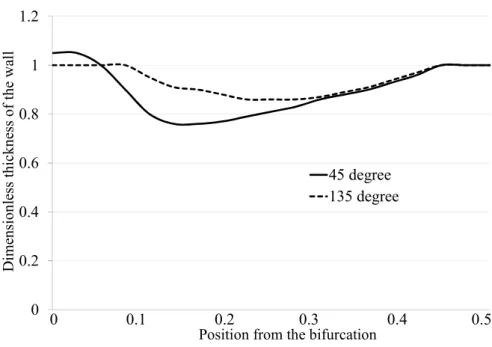
Figure 4 describes thickness of the branch wall around the bifurcation at t = 0.86 s. The transverse axis is the distance from the bifurcation. The longitudinal axis is the thickness of the wall. Thickness = 1.0 means that the wall is not deformed. In the 45 degrees case, the deformation occurs on the upper wall,
(a) Branch angle: 45degrees (b) Branch angle: 135degrees Fig. 3 Enlargement of the branch part (t = 0.86 s)
Fig. 4 Thickness of the branch wall at t = 0.86 s.
0 0.2 0.4 0.6 0.8 1 1.2 45 degree 135 degree
Position from the bifurcation
D im ens ion le ss thi ckn es s of the w al l 0 0.1 0.2 0.3 0.4 0.5
and in the 135 degrees case, it occurs on the lower wall. In Fig.3 and 4, the necessity of hyperelastic consideration in calculation is indicated.
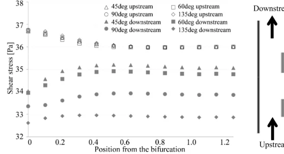
Figure 5 shows shear stress distribution on the right wall of the main vessel at t = 0.86 s. Upstream of the branch, shear stress elevates with increasing closeness to the branch despite the branch angle. Downstream of the branch, shear stress variance is the same between branch angles. However, the shear stress is inversely proportional to the branch angle.
Figure 6 shows the shear stress distribution on the four type of branch angle. Besides, it shows the comparison between the hyperelastic and solid models. At 45 and 60 degree, the shear stress on the wall of the upstream region decreased and that of downstream region increased as the distance from the branch increased. At 90 degree, the shear stress on both walls decreased. On the contrary of the 45 and 60 degree cases, the shear stress increased on the upstream wall and decreased on the downstream wall. In all cases, the flow went from the main pipe into branch with smaller diameter. At 45 degree, the flow near the upstream wall of the branch goes smoothly and the velocity gradient gets calmed gradually. On the contrary, at 135 degree, the flow near the upstream wall of the branch is made go to the almost inverse direction. For that reason, the velocity gradient becomes smaller and gets increased according to straightening of the flow.
Moreover, the shear stress is overestimated in the case of the solid model of both branch angles. Fig. 5 Shear stress distribution on the main right wall
(Grey colored part in the schematic figure of the branch).
Upstream Downstream
Branch angle
■5. Conclusion
Applying the method for solving structure (blood vessel) and fluid (blood flow) at the same time to the branch pipe, the situation of deformation on the hyperelastic wall in the various branch angle cases are shown in detail. The wall thickness around the bifurcation is deformed larger than 10% comparing with before deformation. Moreover, the difference between the shear stress of hyperelastic and solid case is confirmed. Therefore, the necessity of consideration with hyperelasticity is indicated in the same way as our former paper.
(a) 45 degree and 60 degree.
(b) 90 degree and 135 degree.
Fig.6 Shear stress distribution on the branch wall at t = 0.86 s. (Grey colored part in the schematic of branch)
(UP : upstream side, DOWN : downstream side).
Upstream Downstream
Branch angle
■References
1) K. Miyata and M. Miura, “Echocardiography in coronary artery and Kawasaki Disease”, The Journal of Pediatric Practice, Vol.80, (2017), pp.1582-1588
2) M. Petrunic, N. Drinkovic, R. Stern-Padovan, T. Mestrovic, and D. Lovric, “Thoracoabdominal and coronary arterial aneurysms in a young man with a history of Kawasaki disease”, Journal of Vascular Surgery, Vol.50, (2009), pp.1173-1176.
3) Y. Mitani, “Management of Kawasaki disease in the long-term follow-up period”, Journal of Clinical Laboratory Medicine, Vol.60, (2016), pp.622-625.
4) S. Ogawa and M. Ochi, “Consideration of coronary hemodynamics in Kawasaki disease patients with coronary artery lesions and estimation of hemodynamic change before and after surgical treatment”, Journal of The Japanese Coronary Association, Vol.17, (2011), pp.66-74.
5) A. Saito and T. Kawamura, “Numerical analysis of flow in a hyperelastic circular tube model of a coronary artery”, Theoretical and Applied Mechanics Japan, Vol.63, (2015), pp.9-14.
6) K. Sugiyama, S. Ii, S. Takeuchi, S. Takagi, and Y. Matsumoto, “A full Eulerian finite difference approach for solving fluid-structure coupling problems”, Journal of Computational Physics, Vol.230, (2011), pp.596-627.
7) L. H. Peterson, R. E. Jensen and J. Parnell, “Mechanical properties of arteries in vivo”, Circulation Research, Vol. 8, (1960), pp.622-639.
8) J. D. Bronzino and D. R. Peterson, “Biomedical engineering fundamentals”, CRC Press, (2015), pp.162-163.
9) C. W. Hirt and B. D. Nichols, “Volume of fluid method for the dynamics of free boundaries”, Journal of Computational Physics, Vol.39, (1981), pp.201-225.
10) C. Lally, A. J. Reid, and P. J. Prendergast, “Elastic behavior of porcine coronary artery tissue under uniaxial and equibiaxial tension”, Annals of Biomedical Engineering, Vol.32, (2004), pp.1355-1364.
11) J. D. Humphrey, “Cardiovascular solid mechanics : Cells, Tissues, and Organs”, Springer – Verlag New York, (2002), p.329.
12) G.-S. Jiang and C. -W. Shu, “Efficient implementation of weighted ENO scheme”, Journal of Computational Physics, Vol.126, (1996), pp.202-228.
13) T. Konishi, T. Yamamoto, N. Funayama, H. Nishihara, and D. Hotta, “Relationship between left coronary artery bifurcation angle and restenosis after stenting of the proximal left anterior descending artery”, Coronary Artery Disease, Vol.27, (2016), pp.449-459.
14) Y. Bazilevs, K. Takizawa and T. E. tezduyar, “Computational fluid–structure interaction: Methods and applications”, (2012), Wiley, pp.191-258.
15) D. E. Wesson and B. Naik-Mathuria, “Pediatric trauma: Pathophysiology, diagnosis, and treatment, Second Edition”, CRC Press, (2017), pp.107-120.