STUDY ON TWO PHASE FLOW IN MICRO CHANNEL BASED ON EXPERI- MENTS AND NUMERICAL EXAMINATIONS
Takahiko Kurahashi
1, Reika Hikichi
2and Hideo Koguchi
11
Department of Mechanical Engineering, Nagaoka University of Technology (kuraha- [email protected])
2
Graduate school of Nagaoka University of Technology
Abstract. We discuss on two phase flow in micro channel based on numerical and experi- mental studies. The finite element method using stabilized bubble function element is applied to analyze two phase flow. In addition, CFS model (continuum surface model) is included in numerical computation. In this study, two phase flow consists of pure water and Ethyl acetate is treated, and we investigate validity of numerical solution based on experimental results.
Keywords: Finite element method, Stabilized bubble function element, Micro-channel flow, Two phase flow, CSF model.
1. INTRODUCTION
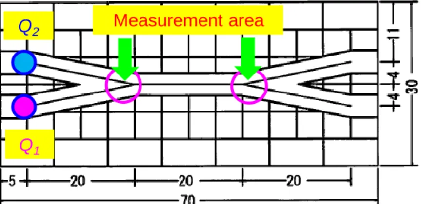
In this study, we focused on macro channel flow in micro chemical chip (See Figure 1.) [1]. It is considered that this chip is widely applicable when we compound a medicine, or carry out environmental analysis, or make emulsions for cosmetics. In case that environmen- tal analysis is carried out by using micro chemical chip, it is necessary to keep two phase flow in micro channel. Hence, the purpose of this study is to construct computational program that is applicable to simulate two phase flow in micro-channel appropriately.
Figure 1. Micro chemical chip
In this study, we employ two fluids, water and ethyl acetate, and temperature of those
fluid is 20 degree. Measurement of interface position is carried out by digital microscope to
compare results by numerical and experimental studies. In numerical study, incompressible
Navier-Stokes equation with CFS model [2] and continuity equation are employed to express flow fields, and advection equation is applied to compute the interface position. The finite element method is applied to compute those equations, and stabilized bubble function element [3] is employed for discretization in space. In addition, fractional step method is applied to compute flow field.
In this study, we focus on Y-junction part for upstream and downstream sides in micro chemical chip, and numerical simulation of two phase flow is carried out. In addition,
comparison with measurement result is also carried out to confirm the validity of result of numerical simulation.
2. GOVERNING EQUATION
In this study, Navier-Stokes equations shown in Equations (1) and (2) are applied to compute flow field.
ij ji
j iV ij i j
i VV P V V f
V
, , , , ,
1
, (1)
,i
0
V
i, (2)
where V
i, P , , and
V
f
iindicate velocity components, pressure, density, viscosity
coefficient and body force per unit volume. In two phase flow, interface position is given by solution of the following advection equation,
,
0
V
i
i
, (3)
and two kind of fluids are separated by value of index function . Fluid properties , are expressed by those of two fluids
(n),
(n)(n=1,2) and index function such as
1
(1)
(2) , 1
(1)
(2). Here, in case of 0 and 1 , fluid properties ,
indicate
(1),
(1) and
(2),
(2) , respectively.
In addition, the CFS model [2] is employed as the interface tension model. Interface or surface tension is given by Equation (4).
] [
,i V
f
i
, (4)
where and indicates interface or surface tension coefficient and curvature, and curvature
is expressed as Equation (5).
iii
i
n
n
, ,
1 n
n
n
(5)
where n
iindicates direction cosine, and is given by the gradient of index function
,i.
3. DISCRETIZATION BY STABILIZED BUBBLE FUNCTION FINITE ELEMENT METHOD
In this study, mixed interpolation is applied to flow field, and bubble function and linear triangle elements are employed for velocity and pressure, respectively. Interpolation functions for velocity and pressure are written as Equations (6) and (7).
4 4 3 3 2 2 1 1
~
i i i i
i NV NV NV NV
V
, (6)
3 3 2 2 1
1
P N P N P
N
P
, (7)
where N indicates shape function, and the shape function is expressed by area coordinate
1,
2,
3 such as N
1
1, N
2
2, N
3
3, N
4 27
1
2
3. It is well known that numerical viscosity can’t be given enough, even if bubble function element is applied. Therefore, the stabilization parameter
BubbleMom.for bubble function element shown in Equation (8) is proposed [3], and this parameter is derived such that stabilization parameter in the SUPG method shown in Equation (9) is equivalent to that in the FEM using bubble function element.
i i eMo m Bu b b le
A d N N
d N
e e
, 4 , 4
2
4 .
, (8)
2 1 2
2 2
2 4
h h
U
S UPG
, (9)
where and indicate numerical viscosity parameter and area of element, and the stabilization parameter is only operated at bubble function point in element, i.e., this parameter is included in 4 , 4 component in viscosity matrix of finite element equation in case of 2D problem. The equation expressed by 4 , 4 component in viscosity matrix is expressed as Equation (10).
2 22 2
4 ,
4 , 4
2 4 1
h h
d U A N
d N N
e
e e
i i
, (10)
where U and h indicate magnitude of velocity in each element and mean element length, and
h is given by
2Ae. In addition, interpolation functions for index function is written as Equation (11).
4 4 3 3 2 2 1 1
~
N N N N, (11)
In the finite element equation for the advection equation, numerical viscosity shown in Equation (12) is added at the bubble function point.
2 2
4 ,
4 , 4
1 2
hd U A N
d N N
e
e e
i
i, (12)
4. DISCRETIZATION BY STABILIZED BUBBLE FUNCTION FINITE ELEMENT METHOD
4.1. Examinations of interface position at junction point for upstream side In this study, comparison of numerical and experimental results is carried out.
Observation area in micro chemical chip is shown in Figure 2. The finite element mesh shown in Figures 3 and 4 and computational conditions shown in Table 1 are employed in numerical study. As the boundary condition for Navier-Stokes equation, inflow boundary condition, i.e.,
0 and
ˆ , ,
0 ˆ ,
) 2 ( )
2 ( ) 2 ( )
1 ( ) 1 ( ) 1
( x y x x y
x V V V V V
V
, is given on
1, wall boundary condition, i.e.,
0 and
, 0 ,
0 ,
0 (1) (2) (2)
) 1
( y x y
x V V V
V
, is given on
2, and condition on outlet boundary i.e.,
0
P
is given on
3. As the boundary condition for advection equation, boundary condition of index function, i.e.,
(1)
ˆ(1) and
(2)
ˆ(2)is given on
1. In addition, observation of interface position by digital probe micro scope is carried out. Magnification is set 540
diameters. Ethyl acetate (Q
1) and pure water (Q
2) are injected from left side of the chip. Water quantity of ethyl acetate is constant, 10μl/min, and that of pure water is changed 10(Case1), 20(Case2), 50 μl/min(Case 3). Results of interface position between numerical and
experimental examinations are shown in Figure 5 and Table 2. It is found that interface position is appropriately obtained in numerical studies.
Measurement area Q
2Q
1Figure 2. Observation area in micro chemical chip
1
2
3Figure 3. Finite element mesh and definition of boundary condition
Figure 4. Magnified figure of figure 3 at junction point Table 1. Computational condition
Condition Value
Time increment Δt 1.0×10
-7sec
Number of nodes 11,991
Number of elements 23,200
Q
1Ethyl acetate: Density ρ 8.984×10
-7,kg/mm
3Q
1Ethyl acetate : Kinematic eddy viscosity ν 0.557, mm
2/s
Q
2Pure water : Density ρ 9.982×10
-7,kg/mm
3Q
2Pure water : Kinematic eddy viscosity ν 1.004, mm
2/s
Interface tension coefficient σ 6.3×10
-6N/mm
Table 2. Comparison of “b
(1)/ H” between experiment and finite element analysis Experiment
b
(1)/ H
Finite element analysis b
(1)/ H
Case1 : Q
110μl/min, Q
210μl/min 0.496 0.481
Case2 : Q
110μl/min, Q
220μl/min 0.359 0.347
Case3 : Q
110μl/min, Q
250μl/min 0.243 0.296
Case 1: Measurement result (Q
110μl/min, Q
210μl/min)
Case 1: Numerical result (Q
110μl/min, Q
210μl/min)
Case 2: Measurement result (Q
110μl/min, Q
220μl/min)
Case 2: Numerical result (Q
110μl/min, Q
220μl/min)
Case 3 : Measurement result (Q
110μl/min, Q
250μl/min)
Case 3 : Numerical result (Q
110μl/min, Q
250μl/min)
Figure 5. Comparison of observation and numerical results
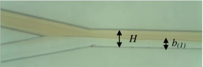
H b
(1)4.2. Examinations of interface position at junction point for downstream side At the downstream side, it is not usual that complete separate interface position is obtained if same flow quantity for two fluids is given. Figure 7 shows the measurement results in case A, Q
1(Ethyl acetate ) 10μl/min - Q
2(Pure water) 10μl/min, and case B, Q
110μl/min - Q
24μl/min. It is found that though two phase flow is separated at Y-junction part for downstream side in case B, that is not clearly separated in case A.
When fluid analysis at only downstream side is carried out, it is necessary to know interface position in parallel flow to give boundary condition on inflow boundary. Therefore, estimation equation of interface position with respect to fluid conditions is derived under an assumption of Couette-Poiseuille flow (See appendix A). Finally, the following estimation equation is derived.
2 3
4
03
2 3
2
4 ) 1 ( 2
) 1 ( ) 1 ( ) 1 ( ) 2 ( 3 ) 1 ( ) 1 ( 2
) 1 ( ) 2 ( ) 1 ( ) 2 ( ) 1 ( ) 1 ( 2 ) 1 (
3 ) 1 ( ) 1 ( ) 1 ( ) 2 ( ) 1 ( ) 2 ( ) 1 ( 4
) 1 ( ) 2 ( ) 2 ( ) 1 ( ) 1 ( ) 2 ( ) 1 (
H q b
H q b
q q q
H
b q q
q H b
q q
, (13)
where lower subscript, ,
H, b and q indicate index of two fluids, kinematic eddy viscosity, width of micro channel, interface height from wall boundary and water quantity per unit length. When Equation (13) is solved, four solutions with respect to interface position b
1are obtained. If the channel width
His considered, the solution can be uniquely determined.
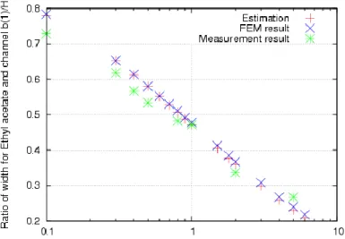
Comparison between measurement results, numerical solutions and exact solutions by Equation (13) is shown in Figure 6. It is seen that exact solutions by Equation (13) are good agreement with measurement results and numerical solutions at upstream side.
Here, numerical analysis is carried out at downstream side using result of Equation (13).
Computational conditions, i.e., physical properties and so on, are same as those shown in previous section. In this case, inflow condition is given as Q
1(Ethyl acetate ) 10μl/min - Q
2(Pure water) 10μl/min. First of all, examination for mesh division is carried out. Two type meshes are shown in Figure 8. One is a uniform division mesh in x-direction, and the other is partially fine mesh near junction point in x -direction. Figure 9 shows the numerical results around Y-junction point in the two cases. In this analysis, interface position on inflow
boundary is estimated based on the result of the Equation (13). It is seen that difference result is obtained in two cases, better result is obtained in case of type 2. From this result, it can be said that fine mesh in x-direction should be prepared around Y-junction point. Next, in case of mesh of type 2, distribution of index function in whole domain is shown in Figure 10. In this result, another case of inflow condition, Q
1(Ethyl acetate ) 10μl/min - Q
2(Pure water) 4μl/min, is also shown. It is seen that similar solution is obtained comparing to the Figure 7.
Therefore, it can be said that if two phase fluid analysis including continuous duration of
laminar flow in micro channel is carried out, interface position is firstly estimated based on
the Equation (13) and numerical analysis at downstream side should be carried out based on
the boundary conditions including the interface position obtained by the estimation equation.
Figure 6. Relationship between “b
(1)/H” and “q
(2)/q
(1)”
Q2: Pure water 10 μl/min
Q1: Ethyl acetate 10 μl/min
Q1: Ethyl acetate 10 μl/min Q2: Pure water 4 μl/min
(Case A) Q
110μl/min, Q
210μl/min (Case B) Q
110μl/min, Q
24μl/min
Figure 7. Measurement results
Type 1 Type 2
Type 1 Type 2
Figure 8. Comparison of mesh division
Type 1 Type 2
Figure 9. Comparison of distribution of index function
(Case A) Q
110μl/min, Q
210μl/min (Case B) Q
110μl/min, Q
24μl/min
Figure 10. Distribution of index function using mesh type 2
5. CONCLUSIONS
In this study, computational process in which flow computation of two phase fluids at Y- junction part for downstream side can be only carried out was constructed. In numerical study, stabilized bubble function finite element method was applied to spatial discretization. In addition, the CFS model was introduced in the governing equation to express interface tension effect. In experimental study, measurement of interface position by digital microscope was carried out. Moreover, estimation equation of interface position was derived, and validity of the result of interface height was confirmed by comparing results between solution by estimation equation, measurement and numerical results. Conclusions are written as follows.
< Y-junction point for upstream side >
・Result of finite element analysis was good agreement with measurement result.
< Y-junction point for downstream side >
・It was found that even if interface position is center line in middle of channel, it is not usual that two kind of fluid can be divided into two channels, respectively.
・It was found that it is necessary to prepare fine mesh near Y-junction point to obtain high accurate result.
・Appropriate solution could be obtained by setting boundary condition based on the
estimation equation of interface position derived in this study.
APPENDIX
Momentum equation for Couette-Poiseuille flow is written as Equation (A.1).
) 2 , 1 1 () (
) ( 2
) ( 2
)
( i
dx dP dy
V
d i
i i x
i
, (A.1)
where V
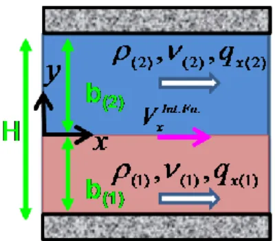
i, P , and indicate velocity components, pressure, density and viscosity coefficient . Figure A.1 shows Definition of two fluids and coordinate system. Boundary conditions for each fluid are written as Equations (A.2) and (A.3).
Figure A.1. Definition of two fluids and coordinate system
0 0
. . ) 1 (
) 1 ( )
1 (
y on V
V
b y on V
Fa Int x x
x
. (A.2)
) 2 ( )
2 (
. . ) 2 (
0
0 b y on V
y on V
V
x Fa In t x x
. (A.3)
General solution for velocity can be represented as Equations (A.4) and (A.5).
. .) 1 ( ) 1 ( ) 2 1 (
) 1 ( ) 1
(
1
2
1
IntFax
x
V
b y y b x y
V P
, (A.4)
. .) 2 ( )
2 ( 2 ) 2 (
) 2 ( ) 2
(
1
2
1
IntFax
x
V
b y y
b x y
V P
. (A.5)
Integrating Equations (A.4) and (A.5), Equations (A.6) and (A.7) are obtained.
Fa In t x
b x
b V dx b
dP dy V q
) . 1 3 (
) 1 ( ) 1 (
) 1 ( 0
) 1 ( )
1 (
2 12
1
) 1 (
, (A.6)
3 (1)
. . )1 ( ) 2 (
) 2 (
. ) . 2 3 (
) 2 ( ) 2 (
) 2 (
0 (2)
) 2 (
2 12
1
2 12
1
) 2 (
Fa In t x Fa
In t x b
x
b V b H
dx H dP
b V dx b
dP dy V q
, (A.7)
Here, if the equilibrium condition for shearing force on interface, i.e.,
(yx1)
yx(2), is considered, the equation (A.8) is obtained.
dy dV dy
dVx x(2)
) 2 ( ) 1 ( ) 1
(
. (A.8)
In addition, introducing a condition that pressure gradient for a fluid is equilibrium to that for the other fluid, the equation (A.9) is obtained by the equations (A.4), (A.5) and (A.8).
. .
) 2 (
) 2 (
) 1 (
) 1 ( )
2 ( ) 1
( 2 IntFa
Vx
b b H x P x P
. (A.9)
Substituting the equation (A.9) to the equations (A.6) and (A.7), and arranging by interface velocity
VxInt.Fa., the equation (A.7) is finally obtained.
2 3
4
03
2 3
2
4 ) 1 ( 2
) 1 ( ) 1 ( ) 1 ( ) 2 ( 3 ) 1 ( ) 1 ( 2
) 1 ( ) 2 ( ) 1 ( ) 2 ( ) 1 ( ) 1 ( 2 ) 1 (
3 ) 1 ( ) 1 ( ) 1 ( ) 2 ( ) 1 ( ) 2 ( ) 1 ( 4
) 1 ( ) 2 ( ) 2 ( ) 1 ( ) 1 ( ) 2 ( ) 1 (
H q b
H q b
q q q
H
b q q
q H b
q q