大阪府立大学　学術情報リポジトリ

(1)

Modular equations and class polynomials of

eta-quotients

著者

Yoshimura Shunsuke

内容記述

学位授与大学: Osaka Prefecture University(大阪

府立大学), 学位の種類: 博士(理学), 学位記番号:

論理第84号, 学位授与年月日: 2010-03-31, 指導教

員: 石井伸朗.

(2)

Modular equations and class polynomials of

eta-quotients

Shunsuke Yoshimura

Osaka Prefecture University

(3)

大阪府立大学博士論文

Modular equations and class polynomials of

eta-quotients

大阪府立大学大学院理学系研究科

博士後期課程情報数理科学専攻

吉村俊介

(4)

Chapter 1 Introduction

In elliptic curve cryptosystems, it is important to construct elliptic curves with a required number of points over a finite field. To construct such elliptic curves, we often make use of the reduction of elliptic curves with complex multiplication. The j-invariant of an elliptic curve with complex multiplication is obtainable by solving the modular equations and the class polynomials of the j-invariant function J over a finite field. However, we have a problem on practical use that the coefficients of these modular equations and class polynomials can be very large. To overcome the problem, one tries to find new modular equations and class polynomials with small coefficients by using some modular functions other than J , for examples, the Dedekind η function.

Besides the application to the theory of elliptic curve cryptosystems, origi-nally the modular equations have been studied as defining equations of modu-lar curves to know their geometric properties. The modumodu-lar curves are moduli spaces of classifying elliptic curves with some properties. Their defining equa-tions are obtained from the algebraic relaequa-tions between the generators of the modular function fields associated with them. To obtain an easily computable defining equation, we have to construct good generators of the modular func-tion field.

One of the important problems in the class field theory is to construct generators of class fields by values of certain (modular) functions. The complex multiplication theory shows that any class field over an imaginary quadratic

(6)

field K is generated by the invariant and coordinates of torsion points of an elliptic curve with complex multiplication by K. In particular, for a ring class field over K, it is generated by a value J (z) of the function J at an imaginary quadratic point z of the complex half plane H such that K = Q(z). We use a class polynomial to compute such a value J (z). Since its coefficients can be very large, it is not easy to obtain a value of J from a class polynomial. Thus one has tried to find a good modular function other than J such that its singular values are class invariants and the related class polynomials are easily computable. We remark that a value f (z) of a modular function f at an imaginary quadratic point z ofH is said to be a singular value of f and that a singular value f (z) is said to be a class invariant if f (z) generates a ring class field over K =Q(z).

Therefore the study of modular equations and class polynomials related to modular functions has been important and has been done continuously since the ages of H.Weber, F.Klein and R.Fricke.

Our purpose of this thesis is to construct some modular functions from

η-quotients and to study the properties of the modular equations and the class

polynomials related to them. The contents of this thesis are as follows. In Chapter 2, we give the fundamental deﬁnitions and results used in the Chapters 3 and 4.

In [4], to compute singular values of the function J , Enge and Schertz pro-posed a method of using class polynomials of double η-quotients and modular equations relating J and double η-quotients. Since double η-quotients are not SL2(Z)-invariant, they uses N-systems to calculate class polynomials of

dou-ble η-quotients. By their method, a singular value of J is obtainadou-ble as a root of the polynomial Φ(J ) which is given by substituting a root of the class polynomial in the modular equation. In their work, it is not clear how class polynomials depend on the choice of N-systems and also it takes much time for identifying the claimed singular value among all roots of Φ(J ).

(7)

polynomials of double η-quotients by using normalizers of a modular group Γ0(N ) and propose a method which reduces the amount of computation in the

process to identify the singular value among solutions by giving a condition that a singular value of J is a multiple root of Φ(J ).

For a positive integer N , let X0(N ) be the modular curve associated with

the modular group Γ0(N ). We denote by A0(N ) the modular function ﬁeld

with respect to Γ0(N ) and identify it with the function ﬁeld of X0(N ). As noted

above, it has been a problem to ﬁnd a modular equation with small integral coeﬃcients for the modular curve X0(N ) by constructing suitable generators

of A0(N ). For individual small values of N , many results are known. Further

M¨uller [10] and Enge and Schertz [5] constructed generators by using eta-quotients and gave modular equation with relatively small integral coeﬃcients in the case N is a prime number and N is a product of two prime numbers respectively.

In Chapter 4, for the case N = 4p where p is an odd prime number, we construct some generators of A0(N ) and study properties of the modular

equations obtained from them. To be more precise, in Section 4.1, we deﬁne three modular functions a, g and h ∈ A0(4p) by using η-quotients and in

Theorem 4.4 show that each pair{g, h}, {a, J}, {g, J} and {a, g} are generators of A0(4p). Further we prove that the modular equations obtained from those

generators have integral coeﬃcients. As a corollary to these results, we show that the singular values of the functions a, g and h, thus the values at imaginary quadratic points, are algebraic integers. In Theorem 4.20 of Section 4.2, we show the modular equation obtained from g(τ ) and h(τ ) has properties similar to those of the (classical) modular equation relative to the function J . For the properties of the classical modular equation, see Theorem 11.18 of [3] or Theorem 2.6 of this article. In Section 4.3, we study the class polynomials of the functions g and a with respect to N -systems. In particular, we establish that singular values g(τ0) of the function g are class invariants for integral

(8)

Chapter 2 Preliminary

In this chapter, we shall state results needed in the following chapters without proofs. For details, we refer to Cox [3], Lang [9] and Silverman [14],[15].

2.1 Elliptic curves and Weierstrass equations

Given a ﬁeld K of characteristic diﬀerent from 2 or 3, an elliptic curve E over

K is a curve deﬁned by an equation of the form y2 = 4x3− g2x− g3,

(2.1)

where g2, g3 ∈ K and ∆ = g23− 27g23 ̸= 0. This equation is called the

Weier-strass equation of E.

Given an elliptic curve E over K, we deﬁne E(K) to be the set of solutions

E(K) ={(x, y) ∈ K × K : y2 = 4x3− g2x− g3} ∪ {O}.

The symbolO = [0, 1, 0] is a point of E at inﬁnity. It is known that E(K) is an abelian group by the chord-tangent composition rule with a neutral element

O.

2.2 Isogenies

Let E1 and E2 be elliptic curves over a ﬁeld K. Let K(E1) and K(E2) be the

(9)

morphism ϕ : E1 → E2 satisfying ϕ(O) = O. We say E1 and E2 are isogenous

if there is an isogeny ϕ between them with ϕ(E1)̸= {O}.

Let ϕ be a non-constant isogeny defined over K. Then ϕ induces an injec-tion ϕ∗ of the function fields K(E2) to K(E2) fixing K,

ϕ∗ :      K(E2)−→ K(E1) f 7−→ f ◦ ϕ.

If ϕ is constant, we deﬁne the degree of ϕ to be 0; otherwise we say that ϕ is

ﬁnite, and deﬁne its degree by

deg ϕ = [K(E1) : ϕ∗K(E2)].

We denote by Hom(E1, E2) the set of isogenies of E1 to E2. An isomorphism

between two elliptic curves deﬁned by Weierstrass equations over K is given by the transformation of (x, y) to (u2_{x, u}3_{y) for u}_{∈ K}×_{. Thus for elliptic curves}

Ei(i = 1, 2) deﬁned by the Weierstrass equation:

y2 = 4x3− g2,ix− g3,i,

E1 is isomorphic to E2 over K if and only if there exists u ∈ K× such that

g2,2 = u−4g2,1 and g3,2 = u−6g3,1. For an elliptic curve E, we put End(E) =

Hom(E, E) and call End(E) the endomorphism ring of E. The invertible elements of End(E) form the automorphism group of E, which is denoted by Aut(E).

If E1 and E2, E are deﬁned over a ﬁeld K, then we can restrict attention to

those isogenies deﬁned over K. The corresponding groups of isogenies are de-noted with the usual subscripts, thus HomK(E1, E2), EndK(E) and AutK(E).

2.3 Reduction modulo p

Let K be an algebraic number ﬁeld, R the ring of integers of K and p a prime ideal of K. Further v be the normalized p-adic valuation so that v(p) = 1. Let E/K be an elliptic curve given in (2.1). Replacing(x, y) by (u−2x, u−3y),

(10)

Weierstrass equation with A, B ∈ Rp, where Rp is the completion of R with

respect to v. Suppose that the coeﬃcients A, B ∈ Rp and the characteristic of

the residue ﬁeld k = R/pR = Rp/pRp is not 2 or 3. Then the discriminant ∆

satisﬁes v(∆) ≥ 0. The Weierstrass equation (2.1) is called minimal equation

for E at v if v(∆) is minimized subject to A, B ∈ Rp.

Suppose that the Weierstrass equation (2.1) is minimal at v. Let π : Rp → k

be the natural reduction map, and t = π(t) for t∈ Rp. Then we obtain a curve

E deﬁned over k by reducing the coeﬃcients A, B modulo p; E/k : y2 = x3 + Ax + B.

The curve E/k is called the reduction of E modulo p. If ∆ =−16(4A3+ 27B2)̸≡ 0 mod p,

namely E is non-singular, then E is said to have good reduction modulo p. For details, see Chapter VII of [14].

2.4 Elliptic curves over

C

In this section, we shall introduce some fundamental facts of elliptic curves over C. Let H be the complex upper half plane, namely, H = {τ ∈ C|Im(τ) > 0} and for τ ∈ H let Λτ =Z + Zτ be the lattice in C generated by 1 and τ.

The Weierstrass ℘-function relative to Λτ is deﬁned by the series

℘(z; Λτ) = 1 z2 + ∑ ω∈Λτ,ω̸=0 ( 1 (z− ω)2 − 1 ω2 ) .

For any positive integer k > 1, we deﬁne the Eisenstein series G2k(Λτ) by

G2k(Λτ) =

∑

ω∈Λτ,ω̸=0

ω−2k.

Since the series for ℘ is uniformly convergent, we can compute the derivative

℘′(z) = ℘′(z; Λτ) by termwise diﬀerentiation:

℘′(z) =−2 ∑

ω∈Λτ

1 (z− ω)3.

(11)

Further, we have

℘(z + ω; Λτ) = ℘(z; Λτ) for all ω ∈ Λτ, z ∈ C,

and

℘(z; Λτ) = ℘(−z; Λτ).

Thus, the Weierstrass ℘-function is an even elliptic function relative to Λτ. It

is known that the elliptic function ﬁeld relative to Λτ is generated by ℘(z) and

℘′(z) overC. Therefore ℘′(z) is algebraic over the ﬁeldC(℘(z)). The algebraic relation between ℘(z) and ℘′(z) is given by

℘′(z)2 = 4℘(z)3− g2(τ )℘(z)− g3(τ ),

where g2(τ ) = 60G4(Λτ) and g3(τ ) = 140G6(Λτ).

The next proposition shows that a lattice Λτ deﬁnes an elliptic curves over

C via the complex analytic map.

Proposition 2.1. (Proposition 3.6, VI of [14])

Let Eτ/C be a curve deﬁned by

Eτ/C : y2 = 4x3 − g2(τ )x− g3(τ ).

Then the map

ϕ :C/Λτ → Eτ(C)

z 7→ [℘(z), ℘′(z), 1]

is a complex analytic isomorphism of complex Lie groups. In particular the curve Eτ/C is an elliptic curve.

We know that any elliptic curve deﬁned overC is isomorphic to the elliptic curve Eτ for a certain τ ∈ H. The discriminant of Eτ is given by ∆(τ ) =

g2(τ )3 − 27g3(τ )2. Therefore ∆(τ ) ̸= 0 for all τ ∈ H. Further the j-invariant

J (τ ) of Eτ is given by

J (τ ) = 1728g2(τ )

3

(12)

The function J (τ ) onH is called the modular invariant function. It is easy to see that elliptic curves Eτ and Eτ′ are isomorphic if and only if J (τ ) = J (τ′).

For an elliptic curve Eτ, we have

End(Eτ) ∼={α ∈ C : αΛτ ⊆ Λτ}.

This is clearly a subring of C, and note that Z ⊂ End(Eτ). If Z ̸= End(Eτ),

then we know that End(E)⊗ Q is isomorphic to a quadratic imaginary ﬁeld

K and that End(E) is isomorphic to an order O of K. In this case, we say

that E has complex multiplication by O or that E has complex multiplication

by K.

2.5 Complex multiplication and

ring class fields

Let Of be the order of conductor f in an imaginary quadratic ﬁeld K. Let

D be the discriminant ofOf and Hf the (proper) ideal class group ofOf. To

a proper ideal a = [β1, β2] = Zβ1 +Zβ2 of Of, we associate its basis

quo-tient αa = β1/β2 (Im(αa) > 0) and a quadratic form qa(X, Y ) = NK/Q(β1X +

β2Y )/NK/Q(a). It is noted that the basis quotient αa is determined up to

SL2(Z)-equivalence and the form qa(X, Y ) is a primitive quadratic form with

integral coeﬃcients of discriminant D. The followings are well known (see [3]). Let a1 and a2 be proper ideals of Of. We write a1 ∼ a2 if a1 and a2 are in

the same ideal class of Of. Then

a1 ∼ a2 ⇐⇒ αa1 is SL2(Z)-equivalent to αa2

⇐⇒ qa1(X, Y ) is proper equivalent to qa2(X, Y ).

(2.2)

Further the map a 7→ qa(X, Y ) gives rise to a bijection between Hf and the

proper equivalent classes of quadratic forms of discriminant D. Since for an ideal a the value J (αa) is independent on the choice of basis quotients αa, we

shall denote by J (a) the value J (αa).

Class ﬁeld theory tells us that there exists a unique abelian extension Kf/K

(13)

the Artin map induces an isomorphism

σ : Hf −→ Gal(K∼ f/K).

The field Kf is called the ring class field for Of. The ring class field for OK

is called the Hilbert class ﬁeld of K. It is the maximal unramiﬁed abelian extension of K.

Let h(D) be the class number of the order Of. Then we know there

ex-ist h(D) isomorphic classes of elliptic curves with complex multiplication by

Of. They are represented by the elliptic curves with j-invariants J (ai), where

ai (i = 1, . . . , h(D)) are ideals representing all classes of Hf. It is an important

fact that the values J (ai) are algebraic integers, which is deduced from the

classical modular equation. See Section 2.9. The following theorem is the ﬁrst main theorem of complex multiplication. This theorem shows J (ai) generates

Kf over K for each i and J (ai) (i = 1, . . . , h(D)) are conjugate to each other

overQ.

Theorem 2.2. LetOf be the order of conductor f in an imaginary quadratic

ﬁeld K and Hf the ideal class group ofOf. Let a be a proper ideal ofOf. Then

K(J (a)) = Kf and the Galois action of an ideal class of Hf on J (a) is given

by

J (a)σ(b)= J (ab−1) for all a, b∈ Hf.

For the proof, see Section 10.3 of [9]. To calculate the values J (ai), we

consider the polynomial

HD[J ](X) = h(D)_∏

i=1

(X − J(ai))∈ Q[X],

which is the minimal polynomial of J (ai) over Q. The polynomial HD[J ](X)

depends only on D. The polynomial HD[J ](X) is called the Hilbert class

polynomial for the order Of. In Section 2.6 of [15], the following theorem is

proved.

Theorem 2.3. LetOf be the order of conductor f in an imaginary quadratic

ﬁeld K and a a proper ideal ofOf. Then

(14)

The roots of HD[J ](X) ∈ Fp[X] are the j-invariants of the elliptic curves

over Fp with complex multiplication by Of for p prime to D. Furthermore,

by the Deuring lifting theorem, every curve E/Fp with complex multiplication

byOf arises as the reduction of a curve A/Kf with complex multiplication by

Of.

Theorem 2.4. (Deuring lifting theorem) Let E/Fp be an elliptic curve with

α ∈ End_F_p(E). Then there exist an elliptic curve A deﬁned over a number

ﬁeld K with β ∈ EndK(A) and a prime p|p of K such that the following is

true. The curve A has good reduction at p. For the reduction A = A mod p, there exists an isomorphism φ : A −→ E, and α corresponds to β under the∼ isomorphism.

For the proof, see Theorem 13.14 of [9]. Hence, an elliptic curve E/Fp has

complex multiplication by Of if and only if j-invariant j(E)∈ Fp is a zero of

HD[J ](X)∈ Fp[X] for a certain discriminant D of an order.

2.6 Dedekind η function

Let z be any complex number of H and put q = exp(2iπz). Dedekind η function is deﬁned by η(z) = q1/24 ∞ ∏ n=1 (1− qn). We can expand η as η(z) = q1/24 ( 1 + ∞ ∑ n=1 (−1)n(qn(3n−1)/2+ qn(3n+1)/2) ) .

It is known that ∆(z) = η(z)24_. _{The Weber functions are example of}

η-quotients. Letting ζn stand for exp(2iπ/n), the Weber functions are deﬁned

by f (z) = ζ₄₈−1η((z + 1)/2) η(z) , f1(z) = η(z/2) η(z) , f2(z) = √ 2η(2z) η(z) , and γ2 = f24_{− 16} f8 , γ3 = (f24_{+ 8)(f}8 1 − f28) f8 .

(15)

We can express the modular invariant J by the Weber functions as follows. J (z) = (f 24_{− 16)}3 f24 = (f₁24− 16)3 f24 1 = (f 24 2 − 16)3 f24 2 = γ₂3 = γ₃2+ 1728. We also have the following transformation formulas.

η(z + 1) = ζ24η(z), η(−1/z) = √ z/iη(z) from which ∆(z + 1) = ∆(z), ∆(−1 z ) = z 12_∆(z).

Further by the transformation formula of Eisenstein series Gk(z), we have

J (z + 1) = J (z), J (−1

z ) = J (z).

For the Weber functions, we obtain

f (z + 1) = ζ₄₈−1f1(z), f1(z + 1) = ζ48−1f (z), f2(z + 1) = ζ24f2(z)

and

f (−1/z) = f(z), f1(−1/z) = f2(z), f2(−1/z) = f1(z).

The Weber function f₂24(z) is a generator of the modular function ﬁelds with respect to Γ0(2).

2.7 Modular groups and modular curves

For a positive integer N , let Γ(N ), Γ0(N ) and Γ0(N ) be the subgroups of

SL2(Z) deﬁned by Γ(N ) =      a b c d   ∈ SL2(Z) a− 1 ≡ b ≡ c ≡ d − 1 ≡ 0 (mod N)   , Γ0(N ) =      a b c d   ∈ SL2(Z) c≡ 0 (mod N)   , Γ0(N ) =      a b c d   ∈ SL2(Z) b ≡ 0 (mod N)   .

(16)

A subgroup Γ of SL2(Z) is called a congruence subgroup of SL2(Z) if it

contains Γ(N ) for some N . We remark that Γ(1) = SL2(Z) and Γ0(N ) =

S−1Γ0(N )S with S =  0 −1 1 0  .

LetH be the complex upper half plane and H∗ =H∪P1₍_{Q) = H∪Q∪{i∞}.}

A congruence subgroup Γ acts on H∗ by

γz = az + b cz + d for γ =   a b c d   ∈ Γ, z ∈ H∗_. (2.3)

The quotient Γ\H has the structure of a Riemann surface. We give the quotient Γ\H∗ the structure of a compact Riemann surface by completing Γ\H with the ﬁnitely many Γ-orbits of P1(Q) called the cusps of Γ\H∗. The Riemann surface Γ\H∗ is called the modular curve associated with Γ. We denote by X(N ) and X0(N ) the Riemann surfaces Γ(N )\H∗ and Γ0(N )\H∗

respectively. It is known that the curve X(1) has only one cusp i∞.

For modular curves X(1) and X0(N ), we have the following important

results.

Proposition 2.5. (1) Every non-cuspidal point τ ∈ X(1) corresponds to an

isomorphic class of the elliptic curve Eτ deﬁned by

Eτ : y2 = 4x3− g2(τ )x− g3(τ ),

(2.4)

where g2(τ ) and g3(τ ) are Eisenstein series given in Section 2.4.

(2) Every non-cuspidal point τ ∈ X0(N ) corresponds to an isomorphic class

of a pair of the elliptic curve Eτ deﬁned by (2.4) and its cyclic subgroup

of order N corresponding to the group ⟨_N1⟩ of C/Λτ.

2.8 Modular function fields and class

invari-ants

Let Γ be a congruence subgroup of SL2(Z). A meromorphic function f on H

(17)

(1) f (τ ) = f (γτ ) for all γ =   a b c d   ∈ Γ,

(2) If x is a cusp of Γ, then in a neighborhood of the cusp x, f has Laurent

series expansion:

∞

∑

n=−n0

a(n)tn

where t is a local parameter at the cusp x.

Let A(Γ) be the field generated by all modular functions with respect to Γ. The field A(Γ) is called the modular function field associated with Γ and is an algebraic function field overC. In particular, we denote by A(N) and A0(N )

the modular function ﬁelds with respect to Γ(N ) and Γ0(N ) respectively. It

is known that A(N ) and A0(N ) are identiﬁed with the function ﬁeld of the

modular curve X(N ) and X0(N ) respectively. Let us consider the modular

invariant function J (τ ) given in Section 2.4. Since g2(τ ), g3(τ ) and ∆(τ ) are

holomorphic and ∆(τ ) ̸= 0 for all τ ∈ H, the function J(τ) is holomorphic on H. Since the group SL2(Z) is generated by

 1 1 0 1   and  0 −1 1 0  , the transformation formula in §2.6 shows that J(τ) is a modular function with respect to Γ(1). Since J (τ + 1) = J (τ ), the modular invariant function J (τ ) has the following Fourier series;

J (τ ) = 1 q + 744 + ∞ ∑ n=1 c(n)qn with c(n)∈ Z, (2.5)

where q = e2πiτ_{. Since X(1) is of genus 0 and has only one cusp, this expansion}

shows that A(1) = C(J). Furthermore we know that Γ0(N ) = SL2(Z) ∩

 N 0 0 1   −1 SL2(Z)  N 0 0 1 

. Therefore A0(N ) is the composition of C(J)

and C(JN). Consequently, A0(N ) = C(J, JN) and A0(N ) = C(J, J1

N), where

Ja(z) = J (az) for a∈ Q.

Let K be an imaginary quadratic ﬁeld. For a modular function f and a point τ ∈ H such that K = Q(τ), the function value f(τ) is called a class

invariant if we have

(18)

The Weber functions are examples of functions yielding class invariants [1].

2.9 Classical modular equation

Let m be a positive integer. The classical modular equation (of level m) was introduced by Kronecker more than 100 years ago. It is an algebraic equation between the functions J and Jm. Note Jm is algebraic over C(J)

since A0(m) =C(J, Jm) is an algebraic function ﬁeld over C. In order to give

the classical modular equation, we consider the set of matrices

C(m) =     a b 0 d   : ad = m, a > 0, 0 ≤ b < d, gcd(a, b, d) = 1   . Let σm =  m 0 0 1 

. For a matrix σ ∈ C(m), put S(σ) = σ−1

m Γ(1)σ ∩ Γ(1).

Then S(σ) (σ ∈ C(m)) are distinct to each other and are all cosets of Γ0(N )

in Γ(1). We have [Γ(1) : Γ0(m)] =|C(m)| = m

∏

p|m(1 + 1/p).

The classical modular equation Φm,J(X, Y ) is deﬁned by

Φm,J(X, J ) = ΦJ,Jm(X) =

∏

σ∈C(m)

(X − J(στ)).

Note that degree of Φm,J(X, Y ) in X equals to|C(m)|. The classical modular

equation has following good arithmetic properties.

Theorem 2.6. (1) Φm,J(X, Y )∈ Z[X, Y ].

(2) Φm,J(X, Y ) = Φm,J(Y, X) if m > 1.

(3) If m is not a perfect square, then Φm,J(X, X) is a polynomial of degree

> 1 whose leading coeﬃcient is ±1.

(4) If p is a prime number, then Φp,J(X, Y ) has the Kronecker congruence

relation : Φp,J(X, Y )≡ (Xp− Y )(X − Yp) mod p.

(19)

Corollary 2.7. Let z ∈ H such that Q(z) is an imaginary quadratic ﬁeld.

Then J (z) is an algebraic integer.

Let E be an elliptic curve over C and j the invariant of E. Then the equation Φm,J(j, Y ) determines isomorphic classes of isogenies of E with cyclic

kernel of degree m.

Theorem 2.8. Let E1/C and E2/C be elliptic curves.

Then Φm,J(j(E1), j(E2)) = 0 if and only if there is an isogeny of E1 to E2

whose kernel is cyclic of degree m.

For details, see§3 of Chapter 5 of [9].

For the elliptic curves over ﬁnite ﬁelds, classical modular equations have the similar property.

Theorem 2.9. Let K be an algebraically closed ﬁeld of characteristic p - m

and let E, E′ be two elliptic curves over K. For the classical modular equation

Φm,J(X, Y ), we let Φm,J(X, Y ) ∈ Fp[X, Y ] be its reduction modulo p. Then

there exists an isogeny of E to E′ of degree m with cyclic kernel if and only if we have Φm,J(j(E), j(E′)) = 0.

For this result, we refer to [10]. It is known that there exists an algorithm for computing the classical modular equations. However the classical modular equations have very large integral coeﬃcients. For example, when m = 3, we have

Φ3,J(X, Y ) = X4+ Y4− X3Y3− 22· 33· 9907XY (X2+ Y2)

+215_{· 3}2_{· 5}3_(X3_{+ Y}3_{) + 2}16_{· 3}5_{· 5}3_{· 17 · 263XY (X + Y )}

+2· 34_{· 13 · 193 · 6367X}2_Y2_{− 2}31_{· 5}6_{· 22973XY}

(20)

Chapter 3 N-systems and class polynomials

for double eta-quotients

The contents of this chapter are based on the results obtained in S.Yoshimura, A.Comuta and N.Ishii [16].

3.1 Basic results and definitions

Let η(z) be the Dedekind η-function. For two prime numbers p1 and p2, the

double η-quotient wN(z) of level N = p1p2 is deﬁned by

wN(z) =

η(z/p1)η(z/p2)

η(z)η(z/p1p2)

.

For s = 24/ gcd(24, (p1−1)(p2−1)), the function wsN(z) is invariant under the

modular group Γ0_{(N ) (see [11]). For a divisor Q of N such that gcd(Q,}N Q) = 1

and Q̸= N, set WQ =

(_{−Q N}

y Qx

)

, where x, y ∈ Z and det(WQ) = Q. Then we

know WQis a normalizer of Γ0(N ). Further we denote by WN the Atkin-Lehner

involution ( 0 N

−1 0) . For N -systems N, Enge and Schertz [4] deﬁned the class

polynomials HN(X) of wsN(z). In the following, we shall recall their results.

LetOf be the order of conductor f in an imaginary quadratic ﬁeld K. Let D

be the discriminant ofOf, Hf the (proper) ideal class group of Of and h(D)

the class number of Of. Let Kf be the ring class ﬁeld of K of conductor f .

(21)

a quadratic form AX2 + BXY + CY2. Furthermore, for a quadratic form q = [A, B, C], we put aq = [A,−B+

√ D

2 ] and αq = −B+

√ D

2A . Since the classical

class polynomial HD[J ](X) has large integral coeﬃcient, it is hard to compute

the polynomial for large D. Enge and Schertz [4] gave the method of using the double η-quotient to obtain a class polynomial with small integral coeﬃcients. Since double η-quotient is not SL2(Z)-invariant, the value wsN(αa) depends on

the choice of ideals a and basis quotients in an ideal class. Therefore we must use N -systems deﬁned by Schertz [13].

Definition 3.1. Let N be a set of h(D) primitive quadratic forms [Ai, Bi, Ci]

of discriminant D. we say N an N -system for Of if forms [Ai, Bi, Ci] satisfy

the following conditions:

1. gcd(Ai, N ) = 1, Bi ≡ Bj (mod 2N ), N|Ci for every i, j;

2. the ideals [Ai,−Bi+ √

D

2 ] form a representative system of Hf.

By Theorems 3.1, 3.2 of [4], we have

Theorem 3.2. Assume prime numbers p1 and p2 satisfy the following

condi-tions: 1. If p1 ̸= p2, then (_D p1 ) ,(_pD 2 ) ̸= −1, 2. if p1 = p2 = p, then either (_D p ) = 1 or p|f.

Then there exists an N -system N ={qi} for Of. Further wsN(αqi) ∈ Kf for

every i and ws

N(αqi) are conjugate to each other over K.

Now the class polynomial of ws

N related to the N -system N is deﬁned by

HN(X) =

h(D)_∏ i=1

(X − ws_N(αqi)) .

By Theorem 3.2, we have HN(X)∈ K[X]. Further Corollary 3.1 of [4] gives

Corollary 3.3. Suppose that following conditions hold:

1. If p1 ̸= p2, then (_D p1 ) ,(_pD 2 ) ̸= −1 and p1, p2 - f;

(22)

2. if p1 = p2 = p̸= 2, then (_D p ) = 1 or p|f; 3. if p1 = p2 = 2, then (_D 2 ) = 1, or 2|f, but D ̸≡ 4 (mod 32). Then HN(X)∈ Z[X].

To relate J (aq) and wsN(αq), the modular equation ΦN(X, J ) relating J

and ws_N is used,which is deﬁned by ΦN(X, J ) =

∏

σ

(X − ws_N(σ(z))),

where σ runs over a representative system of the coset decomposition SL2(Z)

modulo Γ0(N ). We know that ΦN(X, J )∈ Z[X, J] by Theorems 7 and 8 of [5].

To obtain elliptic curves with complex multiplication byOf over the ﬁnite ﬁeld

Fq of q-elements, Enge and Schertz use the polynomials HN(X) and ΦN(X, J )

as follows. Assume that q is a prime number which splits completely in Kf.

Then HN(X) splits completely in distinct linear factors over Fq. Let α be a

root of HN(X) mod q. Then for some i, J (ai) mod q is aFq-rational solution of

ΦN(α, J )≡ 0 mod q. To identify J(ai) mod q among the rational solutions jk,

it is necessary to count the number of Fq-rational points of each elliptic curve

Ek with the j-invariant jk. But, in the case ΦN(α, J ) mod q has the degree 2

in J and a multiple root, we can save the process of counting the number of rational points. In section 3.3, we shall consider the condition that ΦN(α, J )

has J (ai) mod q as a multiple root.

3.2 N -systems and class polynomials

In this section, we study the relation between N -systems and class polynomials.

Lemma 3.4. Let {[Ai, Bi, Ci]} and {[Ai′, Bi′, Ci′]} be N-systems for Of.

Sup-pose that [Ai, Bi, Ci] and [A′i, Bi′, Ci′] are proper equivalent for every i. Then

αi = −Bi+ √ D 2Ai is Γ 0_{(N )-equivalent to α}′ i = −B′ i+ √ D 2A′_i if and only if Bi ≡ Bi′

(23)

Proof. Since [Ai, Bi, Ci] and [A′i, B′i, Ci′] are proper equivalent, there exists a matrix M =   a b c d 

 ∈ SL2(Z) such that αi = M (α′i). We have only to

show M ∈ Γ0(N ) if and only if Bi ≡ Bi′ (mod 2N ). Since we have

BiBi′c− 2A′iBid + Dc = −2AiBi′a + 4AiA′ib,

(3.1)

−Bic− Bi′c + 2A′id = 2Aia,

(3.2)

by substituting (3.2) into (3.1), we obtain

a(B_i′− Bi)− 2Cic = 2A′ib.

Since gcd(A′_i, N ) = 1 and N|Ci, we have a(Bi′−Bi)≡ 2A′ib (mod 2N ).

There-fore M ∈ Γ0_{(N ) if and only if B}

i ≡ Bi′ (mod 2N ).

The following result is deduced from Proposition 3 of [13].

Proposition 3.5. Let [A, B, C] be a primitive quadratic form of discriminant

D such that A > 0, gcd(A, N ) = 1 and N|C. Then there exists an N-system N forOf containing [A, B, C]. In particular, for an integer B such that B2 ≡ D

(mod 4N ), there exists an N -system N for Of containing [1, B, (B2− D)/4].

By Proposition 3.5 and Lemma 3.4, we know the class polynomials of double

η-quotient related to N -systems depend only on integers B, considered mod

2N , such that B2 _{≡ D (mod 4N). In the following, we shall ﬁx an N-system}

containing [1, B, (B2− D)/4] and shall denote it by NB and by HB,N(X) the

class polynomial HNB(X) related to the N -system NB.

Lemma 3.6. Assume that p1 and p2 are odd primes. Let N (D) be the number

of integers B mod 2N such that B2 ≡ D (mod 4N). Then

N (D) =      4 if (_pD 1 ) = 1 and (_pD 2 ) = 1, 2 if (_pD 1 ) = 1 and (_pD 2 ) = 0.

Proof. Let us consider the case (_pD

1

)

= 1 and (_pD

2

)

= 1. Then there exists an integer ai such that a2i ≡ D (mod pi) for i = 1, 2. By Chinese reminder

theorem, we see B2 ≡ D (mod 4N) if and only if

(24)

This shows N (D) = 4. The remaining case can be treated similarly.

If N is odd, then we obtain at most N (D) distinct class polynomials of the double η-quotient.

Lemma 3.7. Let B be an integer such that B2 ≡ D (mod 4N).

Then H_−B,N(X) = HB,N(X).

Proof. We know the q-expansion ws_N(z) = ∑anqn is rational, thus an ∈ Q

(see section 3 of [5]). Therefore we have ws N(z) = ∑ anqn = wsN(−z). Since −(−B+√D 2A ) = B+√D 2A and HB,N(X) ∈ Z[X], we have HB,N(X) = HB,N(X) = H_−B,N(X).

Theorem 3.8. Let N (HD) be the number of distinct class polynomials

HB,N(X). Then N (HD) =      1, 2 if (_pD 1 ) = 1 and (_pD 2 ) = 1, 1 if (_pD 1 ) = 1 and (_pD 2 ) = 0.

Proof. Lemmas 3.6 and 3.7 imply that N (HD)≤ N(D)/2. Thus we have the

assertion.

In the case N (HD) = 2, we have two class polynomials HB,N(X) and

HB′,N(X), where B, B′ are integers such that B2 ≡ D (mod 4N), B′ ≡ B

(mod p1) and B′ ≡ −B (mod p2). We shall show HB′,N(X) is obtainable

from HB,N(X) by a simple transformation. We shall use the following

trans-formation formula of the Dedekind η-function (see Theorem 1 of [5]).

Theorem 3.9. Let M =

 a b

c d



 ∈ SL2(Z) be normalized such that c ≥ 0,

and d > 0 if c = 0. Write c = γ2λ _{with γ odd; by convention, γ = λ = 1 if}

c = 0. Then η(M z) = ϵ(M )√cz + dη(z) with R(√cz + d) > 0, ϵ(M ) = ( a γ ) ζab+c(d(1−a 2₎_{−a)+3γ(a−1)+}3 2λ(a 2₋₁₎ 24 .

(25)

Lemma 3.10. Let Wp1 =

(_−p

1 N

y −p1x

)

with y > 0, y ≡ 1 (mod 2) and p1x−

p2y = 1. Then ws_N(z)ws_N(Wp1(z)) = ( p1 p2 )s . Proof. By Theorem 3.9, wN(Wp1(z)) = wN( −p1z + N yz− p1x ) = η( −z+p2 yz−p1x)η( −p1(z/N )+1 p2y(z/N )−x) η(−p1(z/p1)+p2 y(z/p1)−x )η( −(z/p2)+1 p2y(z/p2)−p1x) = ( p1 p2 ) ζ(1−p2)(1−p1)(1+4y−xy(p1+1)) 24 wN(z)−1.

Since s(p1− 1)(p2− 1) ≡ 0 (mod 24), we have our assertion.

Proposition 3.11. Suppose that

( D p1 ) = ( D p2 ) = 1. Then HB′,N(X) = Xh(D) HB,N(0) HB,N( ( p1 p2 )s /X).

Proof. Let q = [A, B, C] be a form of the N -system NB. Put Wp1(αq) =

−B′₊√_D

2A′ . Then we see easily that B′ ≡ B (mod p1), B′ ≡ −B (mod p2) and

C′ = (B′2 − D)/4A′ ≡ 0 (mod N). If gcd(A′, N ) > 1, then we shall show

there exists an element γ ∈ Γ0(N ) such that the ﬁrst coeﬃcient A′′ of the quadratic form [A′′, B′′, C′′] corresponding to γWp1(αq) is prime to N . It is

noted by the proof of Lemma 3.4 that B′ ≡ B′′ (mod 2N ) and N|C′′. Since ws_N(γWp1(αq)) = w s N(Wp1(αq)), we have HB′,N(X) = ∏ q∈NB (X−ws_N(Wp1(αq))).

By Lemma 3.10, we have our result. Assume that A′ is not prime to N . Put

γ =

 r N

t 1 

, for integers r, t. Then

γWp1(αq) =

(−rB′− tB′N + 2A′N + 2rtC′) +√D

2(−tB′+ A′+ t2_C′₎ .

Therefore we have A′′ =−tB′+A′+t2C′. Since N|C′, we know gcd(A′′, N ) = 1

if and only if gcd(−tB′ + A′, N ) = 1. Assume N|A′. Then gcd(D, N ) = 1 implies gcd(B′, N ) = 1. Hence we can take r = N + 1, t = 1. Next assume pi|A′ and pj - A′. Then we have pi - B′. Therefore we can take r = pjN + 1,

(26)

3.3 Multiple roots of modular equation

In this section, we assume the conditions in Corollary 3.3. We shall give a condition that for singular values α of double η-quotients the polynomial ΦN(α, J ) of J has a multiple root.

Proposition 3.12. The polynomial ΦN(X, J ) has degree (p1 + 1)(p2 + 1) as

a polynomial of X and has degree s(p1− 1)(p2 − 1)/12 as a polynomial of J.

For τ ∈ C and Im(τ) > 0, the equation ΦN(wsN(τ ), J ) = 0 has two roots J (τ )

and J (WN(τ )). In particular, if J (τ ) = J (WN(τ )), then the equation has a

multiple root.

Proof. The assertion concerning the degree follows from Theorem 9 of [5].

The equation ΦN(wsN(τ ), J ) = 0 obviously has the root J (τ ). Similarly,

J (WN(τ )) is a root of ΦN(wsN(WN(τ )), J ) = 0. By Theorem 2 of [5], we have

ws

N(WN(τ )) = wsN(τ ). Therefore J (WN(τ )) is a root of ΦN(wsN(τ ), J ) = 0.

In the following, we consider a ﬁxed N -system NB. Let q = [A, B, C] ∈

NB. Since WN(αq) = B+

√ D

2(C N)

, the action of WN on the ideal aq is given by

WN(aq) = [C_N,B+ √ D 2 ]. Lemma 3.13. If we set aB = [N,−B+ √ D 2 ], then WN(aq)∼ aqaB.

Proof. Put ω = (B +√D)/2. Since gcd(A, B, C) = 1,

aqWN(aq) = [A, ω][C/N, ω] = [AC/N, (C/N )ω, Aω, Bω]

= [AC/N, ω] = (ω/N )[N, (−B +√D)/2]∼ aB.

Since aqaq∼ 1, this shows the assertion.

Proposition 3.14. Let q = [A, B, C]∈ NB. Then J (WN(αq)) = J (αq) if and

only if there exist u, v∈ Z such that

(3.3) u2− Dv2 = 4N, u− Bv ≡ 0 (mod 2N). Proof. By (2.2) and Lemma 3.13, we have

(27)

Further we know the condition aB ∼ 1 is equivalent to the existence of an element   x y z w   ∈ SL2(Z) such that −B +√D 2N = x(−B+₂√D) + y z(−B+₂√D) + w . (3.4)

Let us assume (3.4). Then we have

zB2+ zD− 2wB = −2xNB + 4Ny, w = xN + zB. (3.5)

From (3.5), we have y = −A_NCz. Therefore, from xw − yz = 1, we obtain

(Bz + 2xN )2− Dz2 = 4N . Now, we put u = Bz + 2N x, v = z. Then we have

u2− Dv2 _{= 4N and x =} u−Bv

2N . Further, since x ∈ Z, we have u − Bv ≡ 0

(mod 2N ). Conversely, let u, v be integers satisfying (3.3). Put x = u−Bv_2N ,

y = −AC_Nv, z = v and w = xN + zB. Then we have xw− zy = 1 and

(3.4).

Immediately from Proposition 3.14, we obtain

Corollary 3.15. If J (WN(aq)) = J (aq), then N >−D/4.

Proof. The condition (3.3) shows D = u2−4N_v2 >−4N.

Proposition 3.16. Assume there exist u, v ∈ Z satisfying (3.3). Then the

equation ΦN(wsN(αq), J ) = 0 has a multiple root J (aq).

Proof. The assertion is obvious.

Theorem 3.17. Let aqi (i = 1, . . . , h(D)) be the ideals associated with the

quadratic forms qi = [Ai, Bi, Ci] of NB. Then

J (aq1) = J (WN(aq1))⇔ J(aqi) = J (WN(aqi)) (i = 1, . . . , h(D)).

Proof. Since B1 ≡ Bi (mod 2N ), our assertion follows from Proposition 3.14.

Corollary 3.18. Let ℓ be a prime number which splits completely in Kf. Let

B be an integer such that there exist integers u and v satisfying (3.3). Then for any q∈ NB, ΦN(wsN(αq), J ) has a multiple root J (aq) over Fℓ.

(28)

3.4 Example

We give an example for the result given in Corollary 3.18. Let D =−56 and

N = 39. The integer B = 10 satisﬁes B2 ≡ D (mod 4N) and for u = 10, v = 1

the condition (3.3) holds true. By routine computation, we have

H10,39(X) = X4− 2X3− X2+ 2X− 1, Φ39(X, J ) = X56+ 55

∑

i=0

aiXi,

where coeﬃcients ai are given in the following table:

i ai i ai i ai 55 704− J 54 168568 + 39J 53 14498520− 663J 52 187807764 + 6331J 51 744637296− 35763J 50 −6562036 + 106392J 49 −3840625568 − 18070J 48 1058251610− 1082016J 47 10302034600 + 3516903J 46 4510900472− 1278901J 45 −34331690432 − 18277116J 44 −7097865034 + 40532700J 43 84188024320 + 11574823J 42 546780176− 161476962J 41 −154959173464 + 168751479J 40 −12359340101 + 230086922J 39 327081484064− 617987682J 38 −49301838300 + 137626281J 37 −576339027576 + 928366231J 36 284363953068− 959457720J 35 735938431592− 477589944J 34 −558265224452 + 1429130144J 33 −890017323520 − 466517064J 32 977815434427− 963208272J 31 966995235128 + 909996295J 30 −1755072840368 + 158515461J 29 −345165085024 − 607329720J 28 2218368968890 + 197238236J 27 −911733108784 + 179445279J 26 −1540031876048 − 140684622J 25 1628026178168− 6888479J 24 261124933147 + 37909092J 23 −1229692547200 − 8835450J 22 462040501468− 4070053J 21 441029439032 + 1885689J 20 −422841966612 + 44928J 19 −7261052136 − 111436J 18 163453863300 + 9516J 17 −59787354976 + 740J 16 −26470898021 − 1486J + J2 15 24009911816− 49J 14 −1731574864 + 29J 13 −3926472080 + 246J 12 1333660406− 364J 11 158103088− 221J 10 −172600168 + 650J 9 25597000− 221J 8 5195450− 364J 7 −2155088 + 247J 6 177164 + 26J 5 39936− 52J 4 −9996 + 13J 3 600− J 2 88 1 −16 0 1

It is noted the degree of the Φ39(X, J ) in J is 2. We take a prime number

(29)

607)(X− 166)(X − 3428)(X − 2987) (mod 3593). By substituting the roots of H10,39(X) (mod 3593) into Φ39(X, J ), we have (mod 3593)

Φ39(607, J )≡ (J − 229)2, Φ39(166, J )≡ (J − 2979)2,

Φ39(3428, J )≡ (J − 2874)2, Φ39(2987, J )≡ (J − 2696)2.

On the other hand, the discriminant of Φ39(X, J ) as a polynomial in J is

divided by H10,39(X). This means that the polynomial Φ39(wsN(αqi), J ) has a

multiple root for every from qi ∈ NB, thus, we have J (aqi) = J (W39(aqi)) for

(30)

Chapter 4 Modular equation of a function

field with respect to a group

Γ

₀

(4p)

The contents of this chapter are based on the results obtained in S.Yoshimura, A.Comuta and N.Ishii [17].

4.1 Modular functions

Let η(τ ) be the Dedekind η-function. Given a positive integer δ, we put ϕδ =

ϕδ(τ ) = η(δτ )/η(τ ). Let p be a prime number and m be an integer. Assume

that p≥ 5 and m ≥ 3. We deﬁne three functions a(τ), g(τ) and h(τ) by a(τ ) = ϕ p 2pϕ4 ϕp_4pϕ2 = η(2pτ ) p_{η(4τ )} η(4pτ )p_{η(2τ )}, h(τ ) = ϕ 24 2 ϕ16 4 = η(2τ ) 24 η(τ )8_{η(4τ )}16, g(τ ) = h(mτ ).

(31)

indexed by the positive divisors δ of N such that r1 = 0,            v(i∞) = ₂₄1 ∑_δ_|N(δ− 1)rδ is an integer, v(0) = ₂₄1 ∑_δ_|N(N/δ− N)rδ is an integer, ∏ δ|Nδ rδ _{is a rational square.}

Then the function g = g(τ ) = Πδ|Nϕr_δδ is a modular function with respect to

Γ0(N ).

Proof. See Theorem 1 of [11].

By Theorem 4.1, we have next proposition.

Proposition 4.2. The functions a(τ ), g(τ ) and h(τ ) are modular functions

with respect to Γ0(4p), Γ0(4m) and Γ0(4) respectively.

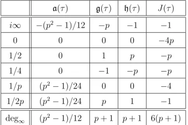
Suppose that m = p in the remaining part of this section. Let f be a modular function with respect to Γ0(N ). We denote by deg_∞f the total

degree of poles of the modular function f on X0(N ). By [12], there exist

six cusps i∞, 0, 1/2, 1/4, 1/p, and 1/2p of Γ0(4p). We give the order of the

modular functions a(τ ), g(τ ), h(τ ) and the modular invariant function J (τ ) at each cusp of Γ0(4p) in Table 4.1.

Table 4.1: the order of the modular functions for Γ0(4p)

a(τ ) g(τ ) h(τ ) J (τ ) i∞ −(p2− 1)/12 −p −1 −1 0 0 0 0 −4p 1/2 0 1 p −p 1/4 0 −1 −p −p 1/p (p2− 1)/24 0 0 −4 1/2p (p2− 1)/24 p 1 −1 deg_∞ (p2_{− 1)/12} _{p + 1} _{p + 1} _{6(p + 1)}

(32)

For a positive divisor d of N and t ∈ Z, consider a matrix Wd,t=   1 t d dt + 1   .

We denote by Wd the set of matrices

{Wd,t| t mod N/ gcd(d2, N )}.

Further, we putW =∪_d_|NWd.

Lemma 4.3. If N = 4p, then the set of matrices W is a system of

represen-tative of the coset decomposition of SL2(Z) with respect to Γ0(N ).

Proof. It is easy to see that any two distinct matrices ofW are not contained

in the same coset and that the order ofW equals to the index [SL2(Z) : Γ0(N)].

Therefore we have the assertion.

We give some generators of A0(4) and A0(4p).

Theorem 4.4. Let h, a, g and J be the functions as above. Then (1) A0(4) =C(h).

(2) A0(4p) =C(a, g) = C(g, h) = C(g, J) = C(a, J).

Proof. Since the modular function h has only one pole on X0(4) and the order

of the pole is equal to one, we see A0(4) =C(h). Thus we have (1). Next we

consider (2). By Table 4.1, we know deg_∞g = p + 1 and deg_∞(a12+ g) = p2. Since gcd(deg_∞g, deg_∞(a12_{+g)) = 1, we obtain A}

0(4p) =C(a, g) from Lemma

2 of [7]. Since Γ0(4p) = Γ0(4)∩ P−1Γ0(4)P, P =   p 0 0 1  

and C(g) is the modular function ﬁeld with respect to P−1Γ0(4)P , we have

A0(4p) =C(g, h) .

Finally we shall prove A0(4p) =C(g, J) = C(a, J). Since A0(4p)⊃ C(g, J),

(33)

representative of the coset decomposition of SL2(Z) with respect to Γ0(N ), it

is suﬃcient to prove g(τ ) ̸= g(Wd,t(τ )) for Wd,t ∈ Γ/ 0(N ). This is immediate

because Table 4.1 shows the q-expansions of g(τ ) and g(Wd,t(τ )) have the

diﬀerent orders. Therefore we have A0(4p) = C(g, J). Similarly we have

A0(4p) =C(a, J).

Let us deﬁne the modular equation for the non-constant functions f and f′ such that A0(N ) =C(f, f′). Since the function f is algebraic overC(f′), there

exists the monic minimal polynomial Φf,f′(X) of the function f over C(f′).

We say Φf,f′(X) the modular polynomial of f relative to f′ and Φf,f′(X) = 0

the modular equation of f relative to f′. In particular, for f ∈ A0(N ) such

that A0(N ) =C(f, J), the modular polynomial Φf,J(X) is given by

Φf,J(X) = ∏ γ∈Γ0(N )\SL2(Z) (X − f(γτ)) = Xψ(N )+ ψ(N )_∑ i=1 Ci,f(τ )Xψ(N )−i,

where Ci,f(τ ) is the i-th elementary symmetric form of f (γτ ). First we show

Φg,J(X), Φa,J(X) ∈ Z[J][X]. To this end, we consider the q-expansions of

g(Wd,t(τ )) and a(Wd,t(τ )) by the transformation formulas of the Dedekind

η-function (see Theorem 3.9).

Theorem 4.5. Let K, K′ ∈ N and T =

 a b

c d



 ∈ SL2(Z) such that c ≥ 0

and d > 0 if c = 0. Write uKa + vK′c = D = gcd(Ka, K′c) and U =

 Ka/D −v K′c/D u  . Then η(KT τ K′ ) = ϵ(U ) √ D K(cτ + d)η ( Dτ + (uKb + vK′d) KK′/D )

with ϵ(U ) as in Theorem 3.9.

Proof. The assertion is obtained from the similar argument in Theorem 3 of

[5]. Letting R0 =  K 0 0 K′   and R =  D uKb + vK′d 0 KK′/D 

, one easily checks that R0T = U R. Thus η(KT τ /K′) = η(R0T τ ) = η(U Rτ ).

(34)

Lemma 4.6. Let us consider an inﬁnite producteg(T, Q) of rational functions

with respect to variables T and Q given by

eg(T, Q) =            24∏∞ n=1 (1−(T Qn₎2₎24 (1−(T Qn₎4₎8₍₁_{−T Q}n₎16 if 2- d, −28_{T Q}∏∞ n=1 (1−(T Qn₎2₎24 (1+T Qn₎8₍₁_{−T Q}n₎16 if 2∥d, (T Q)−1∏∞_n=1₍₁_{−T Q}(1n−(T Q₎8₍₁_{−(T Q}n)2)24n₎4₎16 if 4|d. Then g(Wd,t(τ )) =      eg(ζα+t p , qp) if d = 4, eg(ζ1+dt 4p d , q_βgcd(d,p) d ) otherwise, where α = { 1− ( −1 p ) p } /4, βd = 4p/ gcd(d2, 4p), ζn = exp(2πi/n) and qn = exp(2πiτ /n). In particular, g(Wd,t(τ ))∈ Z[ζ4p]((q4p)).

Proof. Write uδ + vd = D = gcd(δ, d). We put δ0 = δ/D, d0 = d/D and

W0 =  δ0 −v d0 u   . By Theorem 4.5, we have η(δWd,tτ ) = ϵ(W0) √ dτ + dt + 1 δ0 η ( Dτ + v δ0 +D δ0 t ) , η(Wd,tτ ) = ϵ(Wd,t) √ dτ + dt + 1η(τ ). Therefore we obtain ϕδ(Wd,tτ ) = η(δWd,tτ ) η(Wd,tτ ) = ϵ(W0)η ( Dτ +v δ0 + D δ0t ) √ δ0ϵ(Wd,t)η(τ ) .

Let us consider the case d = 1. If δ is divided by p, then we have

ϕδ(W1,tτ ) = ζ₂₄δ−2−tη(τ +1+t_δ ) √ δη(τ ) . This shows g(W1,t(τ )) = ϕ2p(W1,tτ )24 ϕp(W1,tτ )8ϕ4p(W1,tτ )16 = 24 η( τ +1+t 2p ) 24 η(τ +1+t_p )8_η(τ +1+t 4p )16 = 24 ∞ ∏ n=1 (1− ζ_4p2(1+t)q_4p2n)24 (1− ζ_4p4(1+t)q4n 4p)8(1− ζ 1+t 4p q4pn)16 =eg(ζ_4p1+t, q4p).

(35)

Lemma 4.7. Put ea(T, Q) =                          2p−12 ∏∞ n=1 (1−(T Qn₎2₎p₍₁_{−(T Q}n₎p₎ (1−T Qn₎p₍₁_{−(T Q}n₎2p₎ if d = 1, 2, ( 2 p ) ∏_∞ n=1 (1−(T Qn₎2₎p₍₁_{−(T Q}n₎4p₎ (1−(T Qn₎4₎p₍₁_{−(T Q}n₎2p₎ if d = 4, ( 2 p ) 2p−12 (T Q) p2−1 24 ∏∞ n=1 (1−(T Qn)2p)p(1−T Qn) (1−(T Qn₎p₎p₍₁_{−(T Q}n₎2₎ if d = p, 2p−12 (T Q) p2−1 24 ∏∞ n=1 (1−(T Qn₎2p₎p₍₁_{−T Q}n₎ (1−(T Qn₎p₎p₍₁_{−(T Q}n₎2₎ if d = 2p, (T Q)1−p212 ∏∞ n=1 (1−(T Qn₎2p₎p₍₁_{−(T Q}n₎4₎ (1−(T Qn₎4p₎p₍₁_{−(T Q}n₎2₎ if d = 4p. Then _                               a(W1,t(τ )) =ea(ζ4p1+t, q4p), a(W2,t(τ )) =ea(ζ2p1+2t, qp), a(W4,t(τ )) =ea(ζ (1−p)/4+t p , qp), a(Wp,t(τ )) =ea(ζ (−1 p)+t 4 , q4), a(W2p,t(τ )) =ea(−1, q), a(W4p,t(τ )) =ea(1, q). In particular, a(Wd,t(τ ))∈ Z[ζ4p]((q4p)).

Proof. The assertions are obtained from the similar arguments in Lemma 4.6.

For an integer k prime to N , let ψk ∈ Gal(Q(ζN)/Q) be the automorphism

deﬁned by ζψk

N = ζ k N.

Lemma 4.8. Let N = 4p. For a positive divisor d of N and an integer k prime

to N , there exists an integer tk uniquely determined modulo (N/ gcd(d2, N ))

such that g(Wd,t(τ ))ψk = g(Wd,tk(τ )). Further the map: Wd,t 7→ Wd,tk gives

rise to a permutation of Wd.

Proof. Consider the case d = 4. Then we see

g(W4,t(τ ))ψk =eg(ζpα+t, qp)ψk =eg(ζpk(α+t), qp).

Thus we have eg(ζpk(α+t), qp) = eg(ζpα+tk, qp) with an integer tk uniquely

(36)

g(W4,tk(τ )) and the map W4,t 7→ W4,tk is a permutation ofW4. Next, consider

the case d̸= 4. Then we see g(Wd,t(τ ))ψk =eg(ζ1+dt4p d , qgcd(d,p)_β d ) ψk ₌eg(ζk(1+dt) 4p d , q_βgcd(d,p) d ).

Thus we have eg(ζk(1+dt)4p

d , q_βgcd(d,p) d ) = eg(ζ 1+dtk 4p d , qgcd(d,p)_β d ) with an integer tk

uniquely determined modulo βd such that tk ≡ {k(1 + dt) − 1} /d mod βd.

Obviously g(Wd,t(τ ))ψk = g(Wd,tk(τ )) and the map Wd,t 7→ Wd,tk is a

permu-tation ofWd.

Lemma 4.9. Let N = 4p. For a positive divisor d of N and an integer k prime

to N , there exists an integer tk uniquely determined modulo (N/ gcd(d2, N ))

such that a(Wd,t(τ ))ψk = a(Wd,tk(τ )). Further the map: Wd,t7→ Wd,tk gives rise

to a permutation of Wd.

Proof. The assertion is obtained from the similar argument in Lemma 4.8.

Theorem 4.10. The modular polynomials Φg,J(X) and Φa,J(X) belong to

Z[J][X].

Proof. Since Ci,g is SL2(Z)-invariant and has no poles on H, we have Ci,g is a

polynomial of J . By Lemma 4.6, we know Ci,g ∈ Z[ζ4p]((q)). Thus we have

Ci,g ∈ Z[ζ4p][J ]. By Lemma 4.8, we see

{g(γτ)ψk _{: γ} ∈ W} = {g(γτ) : γ ∈ W}

for any ψk ∈ Gal(Q(ζ4p)/Q). Therefore we have Ci,gψk = Ci,g, Ci,g ∈ Z[J] and

Φg,J(X)∈ Z[J][X]. The assertion for Φa,J(X) can be deduced similarly from

Lemmas 4.7 and 4.9.

Since Φg,J(X), Φa,J(X)∈ Z[J][X], we can consider these modular

polyno-mials as polynopolyno-mials of X and J . Therefore we write Φg,J(X) = Φg,J(X, J )

and Φa,J(X) = Φa,J(X, J ) for polynomials Φg,J(X, Y ), Φa,J(X, Y )∈ Z[X, Y ].

Corollary 4.11. Let α be an element of H such that Q(α) is an imaginary

quadratic ﬁeld. Then the singular values a(α), g(α) and h(α) are algebraic integers.

(37)

Proof. For the modular invariant function J , the singular value J (α) is an

al-gebraic integer. By Theorem 4.10, Φa,J(X, J (α)) and Φg,J(X, J (α)) are monic

polynomials whose coeﬃcients are algebraic integers. Thus a(α) and g(α) are algebraic integers similarly. Since h(τ ) = g(τ /p), we see h(τ ) is a root of Φg,J (τ /p) = 0 and Φg,J (τ /p) ∈ Z[J(τ/p)][X]. Since J(τ/p) is an algebraic integer,

h(α) is an algebraic integer.

In the following, we show that the modular polynomial Φa,g(X)∈ Z[g](X).

Let d be a positive divisor of p. For an integer a such that gcd(a, d) = 1, we select a pair of integers (b, v) such that dv− 4ab = 1. For t ∈ Z, put

Bd,t =



d a + dt 4b v + 4bt



 . Then Bd,t ∈ SL2(Z). We denote by Bd the set of

matrices {Bd,t|t mod p/d}.

Lemma 4.12. Let W′ = ∪_d_|pBd and Γ(4, p) = P Γ0(4p)P−1, where P =

  p 0

0 1 

 . Then the set of matrices W′ _{is a system of representative of the}

coset decomposition of Γ0(4) with respect to Γ(4, p).

Proof. The number of elements ofW′ is p + 1. This is equal to [Γ0(4) : Γ(4, p)].

It is easy to see that any distinct matrices in the set W′ are not in the same coset.

Set a∗(τ ) = a(τ /p). To prove Φa,g(X)∈ Z[g](X), we consider the modular

polynomial Φa∗,h(X) instead of Φa,g(X).

Lemma 4.13. Put ea∗_{(T, Q) =}      (T Q)1−p212 ∏∞ n=1 (1−(T Qn₎2p₎p₍₁_{−(T Q}n₎4₎ (1−(T Qn₎4p₎p₍₁_{−(T Q}n₎2₎ if d = 1, ( 2 p ) ∏_∞ n=1 (1−(T Qn₎2₎p₍₁_{−(T Q}n₎4p₎ (1−(T Qn₎4₎p₍₁_{−(T Q}n₎2p₎ if d = p. Then      a∗(B1,t(τ )) =ea∗(ζp1+t, qp), a∗(Bp,t(τ )) =ea∗(1, q). In particular, a∗(Bd,t(τ ))∈ Z[ζp]((qp)).

(38)

Proof. The assertions are obtained from the similar arguments in Lemma 4.6.

Lemma 4.14. For a positive divisor d of p and an integer k prime to p,

there exists an integer tk uniquely determined modulo (p/ gcd(d2, p)) such that

a∗(Bd,t(τ ))ψk = a∗(Bd,tk(τ )). Further the map: Bd,t 7→ Bd,tk gives rise to a

permutation of Bd.

Proof. The assertion is obtained from the similar argument in Lemma 4.8.

Lemma 4.15. A modular function on X0(4) that has only one pole at i∞ is

a polynomial in h(τ ).

Proof. Let f (τ ) be a modular function on X0(4) that has only one pole at i∞.

Its q-expansion has only ﬁnitely many terms with negative powers of q. The

q-expansion of h(τ ) is h(τ ) = 1 q + ∞ ∑ n=0 cnqn,

where the coeﬃcients cn are integers for all n ≥ 0. This shows we can ﬁnd a

polynomial A(x) such that f (τ )− A(h(τ)) is holomorphic at i∞. Since it is also holomorphic on H, it is constant. Thus f(τ) is a polynomial in h(τ).

Since Γ(4, p) = P Γ0(4p)P−1, P =   p 0 0 1  

and A0(4p) =C(a, g) by Theorem 4.4, we see C(a∗, h) is the modular function

ﬁeld with respect to Γ(4, p). Noting A0(4) =C(h), the modular polynomial a∗

relative to h is given by Φa∗,h(X) = ∏ γ∈W′ (X − a∗(γτ )) = Xp+1+ p+1 ∑ i=1 Ci,a∗(τ )Xp+1−i,

where Ci,a∗(τ ) is the i-th elementary symmetric form of a∗(γτ ).

大阪府立大学 学術情報リポジトリ

Modular equations and class polynomials of

eta-quotients

著者

Yoshimura Shunsuke

内容記述

学位授与大学: Osaka Prefecture University(大阪

府立大学), 学位の種類: 博士(理学), 学位記番号:

論理第84号, 学位授与年月日: 2010-03-31, 指導教

員: 石井伸朗.

Modular equations and class polynomials of

eta-quotients

Shunsuke Yoshimura

Osaka Prefecture University

大阪府立大学博士論文

Modular equations and class polynomials of

eta-quotients

大阪府立大学大学院 理学系研究科

博士後期課程 情報数理科学専攻

吉村 俊介

Contents

Chapter 1

Introduction

Chapter 2

Preliminary

2.1

Elliptic curves and Weierstrass equations

2.2

Isogenies

2.3

Reduction modulo p

2.4

Elliptic curves over

C

2.5

Complex multiplication and

ring class fields

2.6

Dedekind η function

2.7

Modular groups and modular curves

2.8

Modular function fields and class

invari-ants

2.9

Classical modular equation

Chapter 3

N-systems and class polynomials

for double eta-quotients

3.1

Basic results and definitions

3.2

N -systems and class polynomials

3.3

Multiple roots of modular equation

3.4

Example

Chapter 4

Modular equation of a function

field with respect to a group

Γ

0

(4p)

4.1

Modular functions

大阪府立大学　学術情報リポジトリ

大阪府立大学大学院理学系研究科

博士後期課程情報数理科学専攻

吉村俊介

₀