Proving and Solving Semi-definite Programming over Reals (Computer Algebra : Algorithms, Implementations and Applications)

Proving and

Solving

Semi-definite Programming

over

Reals

穴井宏和

パブロ・パリロ

HIROKAZU ANAI PABLO. A. PARRILO

(

株

)

富士通研究所

ETH

FUJITSU LABORATORIES LTD ’ _{Swiss FEDERAL INSTITUTE OF TECHNOLOGY} \dagger

Abstract

Semidefinite Programming (SDP) is aclass ofconvex optimization problems with alinear objective

function andlinear matrixinequality (LMI) constraints. SDP problemshave many applicationsin engi-neering andappliedmathematics. We propose areasonablyfastalgorithmtoproveandsolveSDPexactly

by exploiting the convexity of the SDP feasibility domain. This is achieved by combining asymbolic

algorithmofcylindrical algebraic decomposition (CAD) and alifting strategy thattakes into account the convexityproperties of SDP. Theeffectivenessofourmethod isexamined by applying it tosomeexamples

on QEPCAD and maple.

1Introduction

Semidefinite Programming (SDP) is

one

ofthe recent main developments inmathematical

program-ming, with many applications in engineering problems. In particular, awide variety of questions in

systems and control theory,

as

well as in several other areas,

can

be cast and solved

as

SDPproblems,

that is, optimization problems with alinear objective functionand linear matrix inequality (LMI)

con-straints (see $[2],[6]$). For these reasons, SDP problems

are

of great practical and theoretical interest in

controltheory.

Usually, SDPs

are

solved by usingnumericalpackagesbased on

an

interior point method,hence

obtain-ing

an

approximate solution withfinite precision. In certain applications (for instance, SDP algorithms

based

on

algebraic geometry [9]$)$ orcritical situations, such

as

ill-posed problems, there is areal danger of

arrivingat

an

incorrectanswer; we mayobtain a“numerically” feasiblesolution for

an

infeasibleproblem,

or vice

versa.

Hence it is important to develop methodsof computing the exactfeasible solutionofSDP problems, and that

are

also able todetermine theirinfeasibility exactly. This

can

be accomplished by

a

symbolic optimization method based

on

quantifier elimination (QE). Thedownsides of this approach

are

the badcomputational complexity properties ofgeneric QEalgorithms.

Therefore, in this paper

we

propose areasonably faster algorithm to prove and solve SDP problems

exactly based

on

asymbolic method of cylindrical algeb raic decomposition (CAD)[4], and the careful

exploitation of the convexity of the SDP domain. Moreover,

we

also

assume

that

we

have afeasible interior point

as

anumerical interior point method requires

one.

We examine the performance of

our

*[email protected]

’[email protected]

数理解析研究所講究録 1335 巻 2003 年 97-104

method by solving some examples by using $\mathrm{Q}\mathrm{E}\mathrm{P}\mathrm{C}\mathrm{A}\mathrm{D}^{1)}$ and maple. Our method can be regarded as

aspecialized CAD algorithm for SDP exploiting convexity and

an

initial

interior

point. This could be

generalized to other classesof

convex

programming.

2Semidefinite programming

SDP problems. We briefly show the definitions of LMIs andSDP problems. Asymmetric matrix$A\in$

$\mathbb{R}^{n\mathrm{x}n}$ is positive (semi)

definite

if and only if quadratic forms $x^{T}Ax>0(\geq 0)$ for all$x=(x_{1}, \cdots, x_{n})\in$

$\mathbb{R}^{n}\mathrm{s}.\mathrm{t}$.

$x\neq 0$, where$x^{T}$ stands for the transposeof$x$

.

In the sequel, when $A$ is positive (semi) definite,

we

denote it by$A>d0(\geq_{d}0)$

.

For areal symmetric matrix$A$, _{$A>d0(\geq_{d}0)$} if and only if all eigenvalues

of$A$

are

positive (nonnegative). Alinear matrix inequality (LMI) is amatrixinequalityofthe form

$\mathrm{M}(\mathrm{x})$ _{$=M_{0}+ \sum_{i=1}^{m}$}$XiMi>_{d}0(\geq_{d}0)$ (1)

where $x\in \mathbb{R}^{m}$is the variablevectorand$M_{i}=M_{i}^{T}\in \mathbb{R}^{n\mathrm{X}n}$, $i=0$,

$\ldots$,$m$,

are

given symmetricmatrices.

In general, there

are

three types ofgeneric LMI problems; Feasibility problem, Linear objective $\min-$

imization problem under $LMI$ constraints and Generalized eigenvalue minimization problem (see [6]).

Among them

we

consider the problem of minimizing alinear objective function in avector variable

$x\in \mathbb{R}^{m}$ subject to alinear matrix_$M(x)$,

rninirnize $c^{T}x$

(2)

subject to $M(x)\geq_{d}0$,

where$c\in \mathbb{R}^{m}$

.

Thisproblemis called

Semidefinite

Programming (SDP). Foravector So, if$M(x_{0})\geq_{d}0$,

$x_{0}$ iscalled

feasible.

If there is no feasible solution,

we

say that the problem (2) is

infeasible.

Notice in

particular that the optimal solution is

on

the boundary of the (convex) feasible set. Also, SDP includes

many important optimization problems such

as

linearprogramming,

as

special

cases.

Reducing SDP to QE problems Optimization problems ofminimizing

an

objectivefunction $h(x)$

subjectto

aconstraint

that isafirst-0rder formula$\phi(x)$

are

solvedby usingQE

as

follows: First introduce

anew

indeterminate $z$ assigned to the objective function $h$ and consider the

new

first-0rder formula

$\mathrm{M}(\mathrm{x})z)=\phi\Lambda(z-h\geq 0)$

.

We call the polynomial $z-h$ aobjective polynomial Then the problem

minimizing $h$ subject to $\phi$ is formulated

as

aQE problem $\Phi\equiv$ $\exists x_{1}\cdots$ $\exists x_{n}(\phi’)$

.

Next eliminate all

quantified variables $x_{1}$,$\ldots$,$x_{n}$ to have the resulting quantifier-free formula $\Phi’$ in $z$

.

Then $\Phi’$ gives

a

finite union $M$ of intervals for $z$, which shows apossible rangeof$z$

.

If$M$ is empty, $\psi$ is unsolvable $(i.e$

.

infeasible);if$M$ isunbounded from below, $h$has

no

minimumw.r.t. $\phi$;if$m\in M$ isalowest endpoint of

$M$

,

then $m$ is the minimum value of$z$ w.r.t. $\phi$ (fordetails [10]).

Now

we

showhowSDPproblems

are

reduced toQE problems and solved by using QE techniques.

De-termining (semi)definiteness for areal symmetric matrix

can

beachieved without computingeigenvalues

matrixby usingthe followingwell-knownSylvester’scriterion:

Theorem 1(Sylvester’s criterion)

$\underline{L\mathrm{e}tA=(a_{ij})\in \mathbb{C}^{n\mathrm{x}n}}$be

affermitian

matrix. Then $A$ ispositivesemidefiniteifandonly ifallprincipal

1)_Seehttp:$//\mathrm{w}\mathrm{w}\mathrm{w}$

.

$\mathrm{c}\mathrm{s}$

.

usna.$\mathrm{e}\mathrm{d}\mathrm{u}/\sim \mathrm{q}\mathrm{e}\mathrm{p}\mathrm{c}\mathrm{a}\mathrm{d}/\mathrm{B}/\mathrm{Q}\mathrm{B}\mathrm{P}\mathrm{C}\mathrm{A}\mathrm{D}$.html

14-2

minors of$A$ axenon negativei.e.

$\det A$$(\begin{array}{lll}i_{1}i_{2} \cdots i_{r}i_{1}i_{2} \cdots i_{r}\end{array})\geq 0$,

for$1\leq i_{1}<i_{2}<\cdots<i_{r}\leq n$, $r=1,2$,$\cdots$,$n$, where

(3)

$A$$(\begin{array}{llll}i_{1}i_{2} \cdots \cdots i_{r}j_{1} j_{2} \cdots j_{r}\end{array})$

denotes the$r\cross r$ submatrix of A which consists of$(i_{k},j_{l})$-entriesof$A$, where $1\leq i_{1}<i_{2}<\cdots<i_{r}\leq n$

and$1\leq j_{1}<j_{2}<\cdots<j_{r}\leq n$

.

Bythiscriterion,$A(x)\geq_{d}0$can be reduced to

an

equivalentformulawhich is the conjunctionof$2^{n}-1(\equiv$ $\sum_{r=1}^{n}$ $(\begin{array}{l}nf\end{array}))$ inequalities.

3CAD

algorithm

We briefly sketch the basic ideas of cylindrical algebraic decomposition,

see

[4] for details. Assume

that

we

are

given

an

input formula

$\varphi(u_{1}, \ldots,u_{m})\equiv \mathrm{Q}_{1}x_{1}\ldots$ $\mathrm{Q}_{n}x_{n}\psi(u_{1}, \ldots,u_{m}, x_{1}\ldots x_{n})$, $\mathrm{Q}_{i}\in\{\exists,\forall\}$

.

Let $F$ he the set of polynomials appearing in $\psi$

as

left hand sides of atomic formulas. We say that

$C$$\subseteq \mathbb{R}^{m+n}$ is sign-invariant for_$F$ ifevery polynomial in_$F$has aconstant sign

on

allpoints in $C$

.

Then

$\psi(c)$ is either “true” or “false” for all $c\in C$.

Suppose

we

have afinite sequence$D_{1}$,

$\ldots$,$D_{m+n}$ for $F$ which has thefollowing properties:

1. Each $D_{i}$ is afinite partition of

$\mathbb{R}^{:}$

into connected semi-algebraic cells. For $1\leq j\leq n$ each $D_{m+j}$ is

labeled with $\mathrm{Q}_{j}$

2. $D_{i-1}$ for $1<i\leq m+n$ consists exactly of the projections ofall cells in$D_{i}$ along the coordinateof

the $i$-th variable in _{$(u_{1}, \ldots, u_{m}, x_{1}\ldots x_{n})$}

.

For each cell $C\in D_{\dot{\iota}-1}$

we

can

determine the preimage $S(C)\subseteq D_{i}$ underthe projection.

3. Foreach cell$C$ $\in D_{m}$

we

know aquantifier-ffee formula$\delta c$$(u_{1}, \ldots, u_{m})$ describing this cell.

4. Each cell $C$ $\in D_{m+n}$ is sign-invariant for $F$

.

Moreover for each cell $C$ $\in D_{m+n}$ we

are

given atest

point$tc$ in such aform that

we can

determine the sign of$f(tc)$ for each $f\in F$ and thus evaluate

$\varphi(t_{C})$

.

Thenafinitepartition$D_{m+n}$ of$\mathbb{R}^{m+n}$ for_$F$iscalled

an

_$F$-invariant cylindrical algebraic decornposition

of$\mathbb{R}^{m+n}$

.

Aquantifier-free equivalentformula

$\varphi$isobtained

as

the disjunction of all$\delta c$forwhich$C\in D_{m}$

is valid inthe following

sense:

1. For $m\leq i<m+n$,

we

have $D_{i+1}$ that is labeled:

(a) If$D_{i+1}$ islabeled “$\exists"$, then $C\in D_{i}$ is validifat least

one

$C’\in S(C)$ isvalid.

(b) If$D_{:+1}$ is labeled $‘\forall’$, then $C$$\in D_{i}$ is valid if all$C’\in S(C)$

are

valid.

2. Acell$C\in D_{m+n}$ is validif$\varphi(tc)$ is “true.

The algorithm to obtain suchasequence$D_{1}$,$\ldots$,$D_{m+n}$, the quantifier-free formula

$\delta_{C}$, and the test

point$tc$ consistsoftwophases, the projection phaseand construction (lifting) phase.

Projection phase In the projectionphase,oneconstructs from$F\subseteq \mathbb{R}[u_{1}, \ldots, u_{m}, x_{1}, \ldots, x_{n}]$

anew

fi-nite set$F’\subseteq \mathbb{R}[u_{1}, \ldots , u_{m}, x_{1}, \ldots, x_{n-1}]$ whichsatisfies the following condition: Consider_$a$,$b\in \mathbb{R}^{m+n-1}$

such that for all $f’\in F’$the signs of both $f’(a)$_,$f’(b)\in \mathbb{R}$

are

equal. Thenfor all_{$f\in F$} the

correspond-ing univariate polynomials $f(a, x_{n})$,$f(b, x_{n})\in \mathbb{R}[x_{n}]$ both have the

same

number ofdifferent real and

complexroots. This guarantees thefollowingproperty called “_{$delineabilit \oint$}’_{: Let $C$}

beaconnected subset

of$\mathbb{R}^{m+n-1}$ that is sign-invariant for _$F’$

.

For each

$f\in F$ consider the functions $\rho_{k}$

:

$Carrow \mathbb{R}$ assigning

to $a\in C$ the $k$-th real root of$f(a, x_{n})\in \mathbb{R}[x_{n}]$

.

Then all these $\rho_{k}$ are continuous. Moreover, thegraph

of the various $\rho_{k}$ do not intersect. In otherwords, the order of the real roots does not change

as

they

continuously change their position in the real line.

The step from$F$to$F’$iscalledaprojectionanddenotedby $F’:=PROJ(F)$

.

We callpolynomials in

$F’$ projectionpolynomialsand the irreduciblefactors of projection polynomials of$F’$ projection

factors.

Iterative application of PROJ-0perator leads toafinite sequence

$F_{m+n}$,$\ldots$,$F_{1}$, where $F_{m+n}:=F$, $F_{i}:=PROJ(F_{i+1})$

for

$1\leq i<m+n$

.

PHOJ-0perator computes certain coefficients, discriminants, resultants, and subresultant coefficients

obtainedfrom the polynomials in$F_{i+1}$ and their higher derivatives, regarded

as

univariatepolynomials

in their last variable, which is the $(i+1)$-st

one

in $(u_{1}, \cdots, u_{m}, x_{1}, \ldots, x_{n})$

.

The final set $F_{1}$ contains

univariate polynomials in$u_{1}$

.

Construction phase In the constructionphase first constructapartition $D_{1}$ of thereal line $\mathbb{R}^{1}$

into

finitely many intervals that are sign-invariant for $F_{1}$: The real

zeros

of univariate polynomials in $F_{1}$

define asign

invariant

decomposition of

R.

The partition $D_{1}$ consistsof cells that

are

these

zeros

and

the intermediate

open

intervals. Thus

we

isolate the above

zeros

and find test pointsin each interval.

This procedureiscalled the base phase. For

an

openinterval

we

may choose arational test pointbutfor

azero

ingeneral

we

need

an

exact representation of

an

algebraic number. For $1\leq i<m+n$ the partitions$D_{i}\subseteq \mathbb{R}^{i}$

are

computed recursively: The roots ofall polynomialsin

$F_{i}$

as

univariate polynomials in their last variable

are

delineated above each connected cell $C$ in $D_{:-1}$

.

Thuswe

can

cut the cylinderabove $C$ into finitely many connected semi-algebraic cells. Then $D_{\dot{1}}$ is

a

collection of all these cells arising ffom all cylinders above the cells of$7)_{t-1}$

Consider the lifting from the partition $D_{1}$ of

$\mathbb{R}^{1}$

to apartition $D_{2}$ of

$\mathbb{R}^{2}$

since remaining lifting

procedures until$\mathbb{R}^{m+n}$

are

achieved by repeating the

same

procedure

as

the lifting from$\mathbb{R}^{1}$

to$\mathbb{R}^{2}$

. We

show theconstruction ofthetest points of each cell of$\mathbb{R}^{2}$

belonging tothe cylinder

over

acell $C\in D\mathrm{l}$

with atestpoint $\alpha$

.

First specialize the polynomials in$F_{2}:=PROJ^{m+n-2}(F)$ bythe testpoint$\alpha$of$C$

.

Wethenget aset of univariate polynomials in$u_{2}$ and deal with these polynomials

in

$u_{2}$ in the

same

way

asthe base phase, i.e., root isolation and choice oftest points. The liftingfrom $\mathbb{R}^{1}$

to$\mathbb{R}^{2}$

is regarded

as

theconstruction

of

the secondcomponentofthetest pointsof$D_{m+n}$

.

The Constructionphase produces alist of (indexed) cells and theirtest points. We know which cells

$S(C)$ in$D_{i}$originfrom whichcell$C$ in$D_{\dot{|}-1}$

.

Thisimpliesthat afinite sequence $D_{1}$,$\ldots$,$D_{m+n}$ for$F$has

astructure of atree representation. The first levelof nodes under the root of the tree corresponds to

the cells in $D_{1}$

.

The second levelofnodes stands for the cells in$D_{2}$, i.e., the cylindersover the cells of

$\mathbb{R}^{1}$

.

The leavesrepresentthe cells of$D_{m+n}$ (i.e., CAD of$\mathbb{R}^{m+n}$). Atest pointof the correspondingcell

is storedin each node

or

leaf. To each level of the tree there

are

anumber of projection polynomials$F_{i}$

whose signs define acellwhen evaluated

over

atestpoint.

144

4Aspecialized

CAD for SDP

4.1

Improving CAD

algorithm

Projection phase It is crucially important for the efficiency of CAD construction that the PRO3

operator produces

as

smallasetof polynomials

as

possible, whilestillensuring the cylindrical arrangement

of cells in resulting decomposition. Several improved projection operators have been proposed so far

[8, 7, 3].

The complexity of the projection phase is given by the following: given $r$ irreducible polynomials

ofdegree less than

or

equal to $d$in $N$ variables, then after $N-1$ projection steps

we

have $(r\cdot d)^{2^{O(N)}}$

polynomialsofdegree atmost$d^{2^{O(N)}}$

.

Itisoften the

case

that

we

cannot decrease the number of variables

when

we

reduce the target problem considered to

an

equivalent first-0rder formula. Thus, ideally

we

should produce

an

equivalent inputformulawith fewerpolynomials, and smaller degree.

Construction phase There

are

two devicesto improvetheefficiency ofthe constructionphase:

(1) Avoiding algebraic computation during liftingprocesses: Revisit the extension of$D_{1}$ to $D_{2}$

.

Let

$C$ be acell of$D_{1}$ with atest point $\alpha$

.

Consider all polynomials

fi\^u)

$:=/(\mathrm{a}, u_{2})\in F_{2}$ that

are

not

identically

zero.

Therealrootsof$f(u_{2})’ \mathrm{s}$ determine the test points of each cell of

$\mathbb{R}^{2}$

in the cylinder

over

acell $C$. Let $\beta$be aroot of$f(u_{2})$

.

If the test point $\alpha$ is

an

algebraic number,

we

need computations

over

the algebraic extension field $\mathbb{Q}(\alpha)$ for root isolation. Moreover it is required that the test point

of each cell be avector of algebraic numbers

over

asimple algebraic extension of $\mathbb{Q}$

.

Hence

we

need

to compute aprimitive element $\gamma$ for $\mathbb{Q}(\alpha, \beta)$ and represent the test point $(\alpha, \beta)$ as pairs of elements

of $\mathbb{Q}(\gamma)$

.

Computations

over an

algebraic extension field

are

typically

more

expensive than those

over

$\mathbb{Q}$

.

For the efficiency of the construction phase,

we

should consider the possibility of avoidingthe

use

of

algebraictestpoints.

(2) Pruning unnecessary branches of aCAD tree: In general not every cell in the construction is

actually necessaryfor eliminatingquantifiersin agiven input formula$\varphi$

.

This observation

was

firstmade

andgeneralized to partial CADbyH. Hong [5]. Partial CAD systematicallyexploits the logicalstructure

of the input formula. This greatly reduces the number of cells to be considered. Furthermore

we can

expect to exploitthe specialstructureof the inputformula(e.g., convexity)inorder toprune unnecessary

branchesofaCAD tree.

4.2

Exploiting convexity

of

SDP

The feasibility domain of

an

SDP is

aconvex

set, and this implies several important properties: (i)

the feasible region is aunique connected region. Then (ii) the boundary of the feasible region ofthe

SDP is defined by the determinant polynomial. Moreover,

we

also

assume

that afeasibleinterior point

isavailable (we can removethis assumption, at aslightly higher computational cost). We will

use

these

properties toimprove the CAD algorithms in the sequel. Thenext theorem guarantees (ii):

Theorem 2

Thedeterminantvanisheson the boundaryof thedomain ofpositivesemidefiniteness$of\mathrm{a}$realsymmetric

matrix.

Sketch of the proof: All eigenvalues ofasymmetricmatrix

are

realand by the principal axis theorem

the matrix is positive semidefinite iff all eigenvalues are greater than

or

equal to

zero.

Moreover the

eigenvalues,

as

zeros ofthe characteristic polynomial, depend continuously on the entries of the matrix.

Suppose

now

the values of $x_{i}$

are

such that the matrix is

on

the boundary of its positive semidefinite

domain. Then in every neighborhood of this point there is apoint, where the matrix is not positive

semidefinite, andhence has anegative eigenvalue. So by the continuity of eigenvalues, the matrix must

have azero

as

aneigenvalue at thispoint, and

so

the determinant vanishes. 1

(1) improving projectionphase Asshown in\S 2, $M(x)\geq_{d}0$canbereduced toanequivalent formula

that is the conjunction of$2^{n}-1( \equiv\sum_{\mathrm{r}=1}^{n}(\begin{array}{l}nr\end{array}))$inequalities. Sincethe boundary of thefeasible region of

SDP is apart of the determinant polynomial, it issufficientthat

we

consider,

as

an

input of CAD, aset

consistingof

an

objectivepolynomial$z-c^{T}x$ _{andthe determinant}$\det(M)$of$M$

as an

input setofCAD

to obtainthe testpoint whichprovidesaminimum of the objectivefunction. This greatly improves the

efficiency of the projection phase incontrast to the reduction accordingto Sylvester’s criterion.

(2) improving

construction

phase We construct aCAD for

an

input set $\{z-c^{T}x, det(M(x))\}$ in

order to solve

an

SDP given by (2). After$n-1$ recursive projections we have univariatepolynomials in

$z$. We denote the set oftest pointswhich

are

real roots ofthe univariate polynomials in $z$by$T_{R}$, the set

oftest pointstaken ffom the intervals between theroots by$T_{I}$

.

Since the SDP feasibility domain is convex, the feasibleregion of$z$ is auniqueisolated interval. The

endpoints ofthe feasible interval of$z$correspond to the maximumand minimum of$z$, i.e., the objective

function. We call the left endpoint atruth-boundary cell, which gives the minimum and is contained in

Tr. Suppose that

we

have afeasible interior point $x\circ=$ $(x_{1}^{0}, \ldots, x_{n}^{0})$ ofSDP domain. This is the

same

setting

as

the numerical interior point method for SDP. Then since

we

have afeasiblevalue $z_{0}=c^{T}x_{0}$

of$z$, the feasible interval of$z$ consists ofthe connected cells to the cell containing$z_{0}$

.

Here

we

consider

onlythe

case

$z_{0}\not\in T_{R}$because if$z_{0}\in T_{R}$ then

we can

regard the test point of thenext left interval of$z_{0}$

as

$z_{0}$ and then

we can

proceed inthe

same way as

shown below.

The test points larger than$z0$are notneeded tofind theminimumof$z$

.

We

can

denote the test points

smaller than$z_{0}$

as

follows:

$-\infty<\cdots<s_{l}<r\ell<s_{\ell-1}<r_{\ell-1}<\cdots<r_{2}<s_{1}<r_{1}<s_{0}<r_{0}<z_{0}$,

where$r_{i}\in T_{R}$, $s_{i}\in T_{I}$, andlet $r\ell$be the thetruth-boundary cell, i.e., theminimum of$z$

.

Inorder tofind

the truth-boundary cellwe start with construction ofaCAD ffom

over

the cellwith atest point

so

$\cdot$ If

the cell withatest point $s_{0}$has a“true” leafthen

we

construct

aCAD over

thecell$s_{1}$

.

In other word

we

make depth-firstsearch of “true” leaf oftheCAD tree

over

$s_{i}’ \mathrm{s}$from the right to the left until acertain

$s_{i}$has

no

“true” leaf. We

can

also employ theorder of

$s_{i}’ \mathrm{s}$tobe considered accordingto bisection. Then

we obviouslyhave the following proposition: Proposition 3

There exists

an

integer $\ell$ such that

$s_{\ell-1}$ has a“true” leaf but $s_{\ell}$ hasno “true” leaf then $r_{\mathit{1}}$ is the

truth-boundarycell.

The coordinate $x_{\min}$ which gives the minimum value of $z$

can

be obtained by lifting

over

the truth

boundary cell. Note that

we

do not have to

use

test poins

in

$T_{R}$ to identify which test point

is

the

14-6

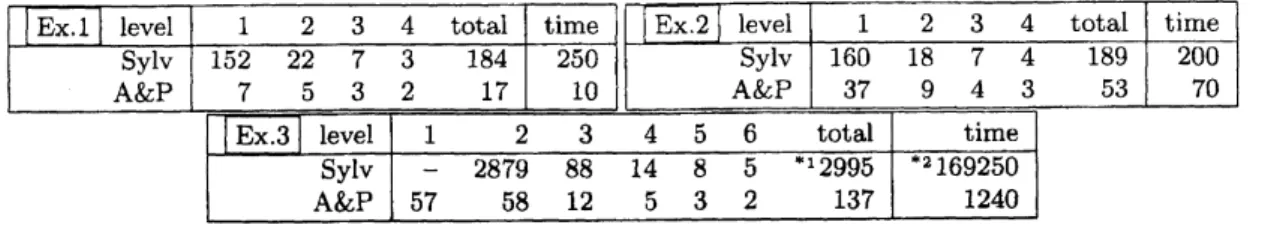
Table 1: Computational results for projectionphase

truth-boundary cell. As for the lifting at the level of the tree corresponding to $x_{i}$,

we can

also prune

unnecessary branchessince the feasible region consistsof the connected cellstothe cell with atest point

$x_{\dot{\mathrm{t}}}^{0}$

.

Thus

we

can

ignore outer both sides ofthe feasibleregion.

5Examples

We have examined how

our

improvementswork for the following SDP problems by using QEPCAD

andmaplefor projection phaseand for constructionphase, respectively. 2)

Example 1. Afeasible interiorpoint is: $(a, b, c)=(0,3,0)$

.

objective: $a+b+c$, $\mathrm{s}.\mathrm{t}$. $\{\begin{array}{ll}1 a 3-ba 5c3-b c9\end{array}\}\geq 0$

.

Example 2. Afeasible interiorpoint is: $(a, b, c)=(1, -1,1)$

.

objective: $a+2b+3c$, $\mathrm{s}.\mathrm{t}$

.

$\{\begin{array}{ll}a bb c+1\end{array}\}\geq 0$, $\{\begin{array}{ll}1 b+cb+c 2-a\end{array}\}\geq 0$

.

Example 3. This example arisesfrom the minimization ofasymmetric quartic polynomial. Afeasible

interior point is: $(\gamma, a, b, c, d)=(60, -1,12,2,4)$

.

$\mathrm{o}\mathrm{b}\mathrm{j}$ective: 7,

$\mathrm{s}.\mathrm{t}$

.

$\{$

$\gamma$ $a$ $b$

$a$ 1 $c$ $b$ $c$ $2d$

$\geq 0$, $1-2a\geq 0$, $\{\begin{array}{ll}2b dd 1\end{array}\}\geq 0$, $2c-3\geq 0$

.

Projection phase: Table 1shows the number of projection factors appearingat eachlevelof the CADtree

and total timetoaccomplish theprojectionphasefor theabovethree examples. Here, $*_{1}$

means

the time

untillevel 2and $*_{2}$

means

thetime untilQEPCAD halted

on

computing level 1. “Sylv”

uses

Sylvester’s

criterion toreduce

an

SDP to afirst-0rder formula and ”A&P’’ is

our

approach shown in the previous

section. Our approach performs much betterthan the approach using Sylvester criterion.

Construction

phase: We applied QEPCADforthe constructionphaseoftheaboveSDPproblemstogetthe

minimum ofobjectivefunctions (withthe$\mathrm{o}\mathrm{p}\mathrm{t}\mathrm{i}\mathrm{o}\mathrm{n}+\mathrm{N}50000000$;asizeforSACLIB’s garbage collected array.

The default value$\mathrm{i}\mathrm{s}+\mathrm{N}2000000$). However, QEPCAD haltedduetolack of memorywithamessage “Too

few cells

reclaimed”

for allexamples. Unfortunately

we

have notyet finished the implementation of

our

proposed method. Wemanually applied the strategy for choosingtestpoints fortheabove examples

$\underline{\mathrm{o}\mathrm{n}\mathrm{m}\mathrm{a}\mathrm{p}\mathrm{l}\mathrm{e}.}$Then

wewere

ableto solvethe constructionphases for all examples inafew minutes.

$2)\mathrm{A}11$the computationsare executedon aPC with aCPU Pentium III lGHz and 756 MB memory.

6Conclusions

We have proposedanefficientalgorithmtocomputean exact (algebraic) representations of the solution

ofSDPproblems. Our approach

can

be regarded

as

aspecialized CAD algorithm for partiallyexploiting

the convexity of SDP andas asuccessful attempt of fusing symbolic and numeric approaches to achieve

efficiency. We hope this work leads to further generalizations of symbolic approaches exploiting convexity

tootherrelated problems.

Amapleimplementationofthe method proposed here

on

top of the SyNRAC-package[1] is planned.

Acknowledgements

The authors would like to thank C. W. Brown for his invaluable help. The authors would like to

thank K. Yokoyama, S. Hara, andV. Weispfenningfor fruitful discussions.

References

[1] H. Anai and H. Yanami. SyNRAC: Amaple-package for solving real algebraic constraints. In

Proceedings

_of

the

International

Workshop

on

Computer Algebra Systems and Their Applications:

CASA’2003. To appear inthe series LNCS, Springer-Verlag.

[2] S. Boyd, L. Ghaoui, E. Feron, and V. Balakrishnan. Linear $Mat\dot{m}$ Inequalities in System and

Control Theory, SIAM Studies in Applied Mathematics, vo115. SIAM, 1994.

[3] C.W. Brown. Improved projection for cylindrical algebraic decomposition. Journal

_of

Symbolic

Computation,

32

(5):447-465,2001.

[4] G.E. Collins. Quantifier Elimination for Real Closed Fieldsby CylindricalAlgebraic Decomposition,

LNCS 32. Springer Verlag, 1975.

[5] G.E.Collins and H. Hong. Partial cylindrical algebraic decomposition for quantifier elimination.

Journal

_of

Symbolic Computation, 12(3):299-328,Sept.

1991.

[6] P. Gahinet, A. Nemirovski,

A.J.

Laub, and M. Chilali. LMI Control Toolbox User’s Guide, For Use

with

MATLAB.

TheMATH WORKS INC, 1995.

[7] H. Hong. An improvement ofthe projection operator in cylindrical algebraic decomposition. In

IS-SAC: Proceedings

_of

the ACM SIGSAM Intemational Symposium on Symbolic and Algebraic

Com-putation,

pages

261-264, 1990.

[8] S. McCallum. An improved projection operation for cylindrical algebraic decomposition of

three-dimensional space. Jourmal

_of

Symbolic Computation, $5(1- 2):141-161$, Feb.-Apr. 1988.

[9] P. A. Parrilo, Semidefinite programming relaxations for semialgebraic problems, Math. Prog. Ser.

B, to

appear, 2003.

[10] V.Weispfenning. Simulation and optimization byquantifier elimination. J. Symbolic Computation,

24(2):189-208,

1997.

148