THREE DIMENSIONAL COMPUTATION OF TAYLOR-COUETTE FLOW(Flow Instability and Turbulence)

(1)

THREE DIMENSIONAL COMPUTATION

OF TAYLOR-COUETTE FLOW

Naoki Matsumoto (松本直樹)

The Institute of Computational Fluid Dynamics, Tokyo, Japan

Susumu

Shirayama (白山晋)

The Institute of Computational Fluid Dynamics, Tokyo, Japan

Kunio Kuwahara (桑原邦郎)

The Institute of Space and Astronautical Science, Tokyo, Japan

1. Abstract

Three dimensional incompressible

Navier-Stokes

equations

are

solved

nu-merically for Taylor-Couette flow with the outer cylinder at rest. The

wave-length of supercritical Taylor vortices created through

an

impulsive start

of the inner cylinder is studied. The evolution of Taylor-vortex structure is

visualized and canbe investigated precisely. The results are compared with

(2)

2. Introduction

Experiments for flows between concentric cylinders

were

performed by

Bur-khalter&Koschmieder (1974). They measured the wavelengths of

steady-statevortices that resulted ffom impulsively starting theinner cylinder from

a state of rest with the outer cylinder held fixed. According to these

exper-iments, the wavelength initially decreased up to $R/R_{c}\approx 4(R_{c}$ : Critical

Reynolds number from linear theory). Beyond $R/R_{c}\approx 4$, the wavelength

increased with increasing$R$

.

The objective of the present work istoexamine

this problem. The visualization and the measurements of the 3-dimensional

flow

are

very difficult, and there

seems

to be

no

current theory available for

such strongly nonlinear flows. Therefore it appears that numerical

simula-tion is the only useful tool for our

purpose.

Neitzel (1984) performed the

axisymmetric computation of the incompressible

Navier-Stokes

equations

in finite-length concentric cylinder geometry. But the wavelength did not

increase for $R/R_{c}>4$

.

So we have performed 3-dimensional computation

and compared the results with the experiments.

3. Numerical Method

Consider a pair of concentric cylinders of radii $a$ and $b$ and height $h$

.

We

assume

the

gap

between the cylinders to be filled with a viscous

incom-pressible fluid of kinematic viscosity $\nu$

.

The entire system is assumed to

be in

an

initial state of rest. At time $t=0$, the inner cylinder at radius

$r=a$ is impulsively set into rotation with angilar velocity $\Omega$ while the outer

cylinder at $r=b$ is held fixed. The rigid endwalls at $z=0,$$h$ are assumed

to be attached to the inner cylinder and therefore begin to rotate with it at

$t=0.The$ variables

are

made dimensionless using the scales $d\equiv b-a,$$\Omega d$

and $\Omega^{-1}$ for length, speed and time respectively.

Numerical method is based

on

the MAC method except treating

pres-sure. The incompressible

Navier-Stokes

equations

are

expressed as follows:

$\frac{\partial v}{\partial t}+(v\cdot\nabla)v=-gradp+\frac{1}{R_{e}}\triangle v$ (1)

divv $=0$ (2)

These equations are written in

a

generalized coordinates system and solved

(3)

sides of equation (l),we obtain the poisson equations for gradient of

pres-sure:

$\triangle P=-grad\cdot div(v\cdot\nabla)v+gradR+rot\cdot$ rotP $(3a)$

where

$R=-\frac{\partial D}{\partial t}+\frac{1}{R_{e}}D$, $P=gradp$, $D=divv$ $(3b)$

and the formula of vector analysis $grad\cdot divX=\triangle X+rot\cdot$ rotX is used.

The time derivative,$\partial D/\partial t$, is evaluated by forcing $D^{n+1}=0$, i.e.,

$\frac{\partial D}{\partial t}\simeq-\frac{D^{n}}{\triangle t}$

The boundary conditions for (1), (3) are

as

follows(dimensional variables):

$u=V$, $v=0$, $w=0$

$P_{r}=\frac{1}{R_{e}}\frac{\partial^{2}u}{\partial r^{2}}+\frac{V^{2}}{a}$, $P_{\theta}=\frac{1}{R_{e}}\frac{1}{a^{2}}\frac{\partial^{2}v}{\partial\theta^{2}}$ $P_{z}=\frac{1}{R_{e}}\frac{\partial^{2}w}{\partial z^{2}}$

at $r=a$

$u=0$, $v=0$, $w=0$

$P_{r}=\frac{1}{R_{e}}\frac{\partial^{2}u}{\partial r^{2}}$ $P_{\theta}=\frac{1}{R_{e}}\frac{1}{b^{2}}\frac{\partial^{2}v}{\partial\theta^{2}}$ $P_{z}=\frac{1}{R_{e}}\frac{\partial^{2}w}{\partial z^{2}}$

at $r=b$

$u=r\Omega$, _$v=0$, _$w=0$

$P_{r}=\frac{1}{R_{e}}\frac{\partial^{2}u}{\partial r^{2}}+\frac{u^{2}}{r}$, $P_{\theta}=\frac{1}{R_{e}}\frac{1}{r^{2}}\frac{\partial^{2}v}{\partial\theta^{2}}$ $P_{z}=\frac{1}{R_{e}}\frac{\partial^{2}w}{\partial z^{2}}$

at $z=0,h$ $(u, v, w)$ are the velocity components in the directions given by the

cylindrical coordinates $(r, \theta, z)$, and ($P_{r}$,P9,$P_{z}$)

are

the components of $P$

in each direction. The Poisson equations for gradient ofpressure

are

solved

by successive

over

relaxation. Dealing with gradient of pressure instead

(4)

and the

convergence

becomes good. The Euler semi-implicit scheme is used

for the time integration of velocity. (All but the convective velocity

are

computed implicitly.) All spatial derivatives except the nonlinear terms

are

approximated by centraldifferences. The nonlinear terms are $app_{f}roximated$

by the third-order upwind scheme:

$(u \frac{\partial u}{\partial x})_{i}=u;\frac{-u_{i+2}+8(u_{i+1}-u_{i-1})+u_{i-2}}{12h}$

$+|u_{i}| \frac{u_{i+2}-4u_{i+1}+6u_{i}-4u_{i-1}+u_{i-2}}{4h}$

We

assume

the flow to be symmetric about the midplane to reduce the

size of the computational domain. This restricts the flow to have an

even

number of vortices, which is the

case

normally observed in the laboratory.

A grid system is shown in fig.l. Constant grid spacing is used in each

direction. The computations

were

done on Japanese supercomputer

NEC

SX2.

4. Results

There are three nondimensional parameters:

$\eta=b/\grave{a}$ (Radius ratio)

$\gamma=h/d$ (Ratio ofheight and gap)

$R_{e}=\Omega d^{2}/\nu$ (Reynolds number)

$(R_{c}=31.03)$

cf) $Ta= \frac{2\eta^{2}}{1-\eta^{2}}R_{e}^{2}$ (Taylor number)

$\eta$ is fixed at 0.727, and $\gamma$ is fixed at

23.35

to correspondwith the experiment

of Burkhalter

&Koschmieder.

The computations

are

performed for four

cases

$R/R_{c}=2,3,4,6$ ($R_{c}:Critica1$ Reynolds number from linear theory).

Steady-state

Figure.2 shows instantaneous streamlines in the vertical surface for $R/R_{c}=$

(5)

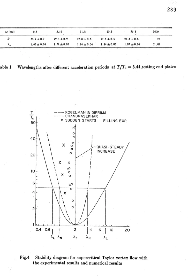
comparison of the experimental and other numerical results. The

wave-length $\lambda$ is defined as follows:

$\lambda=\frac{\gamma-2\epsilon}{N}$

where $\epsilon$is thelength of the endcell,and $N$ isthe number ofvortex-rings$(=1/$

$2$ number of cells) excluding endcells. The agreement is not good

quanti-tatively. Probably the main reason is that the experiment is not a perfect

impulsive start. According to other experiments of them, the wavelength

depends

on

the history of the acceleration.(Table 1) And another

reason

is

from the numerical

error

due to the discontinuity in the boundary

condi-tions at the axial end plates. However wavelengths of computational results

are

within the theoretical limit (Fig.4). The quantitative agreement is not

good, but the agreement is good qualitatively. Both wavelengths of the

computational results and the experiments increase for $R/R_{c}>4$

.

Evolution

_of

Taylor-vortices

Why does the wavelength increase for $R/R_{c}>4$ ? We have investigated

the time-evolution of vortices.

(1) $R/R_{c}=3$

At first, avortex develops from the end-boundary by Ekman pumping,

induces next vortex, and propagates up. Finally vortices fill the

gap

between the cylinders and

go

to the steady-state. Flow is axisymmetric

during this procedure. Fig.$5a$ shows the instantaneous streamlines in

the vertical surface. Fig.$5b$ shows the contour of the vorticity normal

to the surface. It is found that the vorticity is supplied from the inner

boundary.

(2) $R/R_{c}=6$

Vortices fill the

gap

between the cylinders by the

same

process with

case(l). However, this is not the steady-state. This state makes

a

transition to the state in which there

are

large Taylor

vortices.

Fig.$6a$

shows the instantaneous streamlines inthe vertical surface. During the

transition

we

found that wavelengths ofvortices gradually

increase

by

vortex-connection. This feature is not found in the axisymmetric

(6)

So

the transition

are

probably due to the non-axisymmetric effects.

Fig.$6b$ shows the contour of the vorticity normal to the surface. It is

found that the

vortices

which have the

same

sign

are

connecting.

5. Conclusion

The wavelength of Taylor vortices through an impulsive start increases for

$R/R_{c}>4$ by vortex-connection, and this feature

was

not found by

ax-isymmetric computation by Neitzel (1984). So this is the non-axisymmetric

effect.

REFERENCES

[1] S.Chandrasekhar : Hydrodynamic and Hydromagnetic Stability

(Ox-ford University Press,Ox(Ox-ford,1961) p.303

[2] S.Kogelman&R.C.DiPrima : Stability of spatially periodic

supercrit-ical flows in hydrodynamics. Phys.Fluids

13

(1970)

[3]

J.E.Burkhalter&E.L.Koschmieder

: Steady supercritical Taylor

vor-tices after sudden starts. Phys.Fluids 17,1929 (1974)

[4] G.P.Neitzel: Numerical computation of time-dependent Taylor vortex

(7)

GRI

$0$ PO

INT

$S=$ $3\emptyset\star 31\star 1\emptyset 1$

(8)

qコ寸 $e\hat{o}$ $N^{\wedge}$ $11$ $\approx^{o}$ $\sim\approx$ 科 $\cup Q)$ $e_{\frac{t\S}{\Xi\infty}}$ 何 . $\cdot$ $\underline{V}$ $\underline{*\partial}$ $Q)\succ$ $o_{\circ}$ $A^{\Phi}rightarrow$ $11$ $\infty$ . 目 $\downarrow$

1

$\sim_{(l1}\partial$ $\frac{\infty}{O}\Phi$ 邸 $\sim g$ $B\mathfrak{X}$ $-\dot{\infty}$ $Pr$ $11$ $\infty$

(9)

(10)

$\wedgerightarrow$ $\frac{\circ}{..arrow_{\frac{N}{z^{Q)}}}Q)}$ $\overline{\Phi\circ}$ $r\circ\succ$ $SA\Phi$ \={o} $A_{(\lrcorner}$ $+_{\dot{6}}-$ $o\infty$ $-$ $\#$ a $\delta$ 科 $\frac{\overline{\star Q)}}{A^{6}}$ $arrow\frac{\underline{o}}{\Phi^{\partial}}$ 七日 $\overline{v}\approx$ 日 A 家 $\infty b$

$-\underline{a}_{r}\circ\succ$

.

$\frac{rightarrow}{\overline{\Phi tl1}}\cdot\not\in$

臼 $=\sim\backslash \prec 0$

$\frac{o}{P\dashv\succ_{6}}*\underline{\mathfrak{B}}-\#\overline{.e\frac{v}{\frac{}{Q)}}}\frac{+^{\infty}}{-}$ $rn6S$ $ $\underline{\infty\approx}arrow\overline{\Phi}\underline{-}\overline{6}$

$\succ q.\xi+_{\overline{Q)}Q)}\underline{v}$

$\neq_{\frac{b:}{\underline\omega}}c\prec\alpha 0_{E^{\aleph^{)}}}$ 陶 $\frac{a}{z}$

$g_{\wedge-\wedge}^{\succ_{6}\ddot{o}X\bullet}Qj\cdot$ . $\triangleleft mo$ $\dot{}^{\frac{b}{\}}ffeo_{\dot{0}}$ く q $q^{v}$ $\underline{\backslash \approx}$ $11$ トト

(11)

36.4.

$1\overline{v_{m}\overline{\lambda}}$ $30.9\pm 0.7165\pm 0.04$ $29.3\pm 0.91.74\pm 0.05$ $27.8\pm 0.61.84\pm 004$ $27.8\pm 0.51.84\pm 003$ $27.3\pm 0.61.87\pm 004$

2.0425

Table 1 Wavelengths after different acceleration periods at $T/T_{c}=5.44,raeting$end plates

Fig.4 Stability diagram for supercriticalTaylor vortex flow with the experimental results and numerical results

(12)

$^{\backslash }0\backslash |\acute{f}_{\vee}\hat{c})\mathbb{Q}_{1}^{\cap^{\prime\sim_{t}}1r_{C}\perp@^{-}t^{\int_{\backslash }\gamma^{\backslash }}}J’:)\acute{(Q\vee}))r_{-}C^{\wedge})\rfloor\prime^{\wedge\bigwedge_{arrow}}\backslash \prime’*_{\vee^{\wedge\sim}}cu)_{1}^{\backslash \}}|\acute{\overline{\subset}}cJ_{c^{--d\wedge}}|$

$\textcircled{0} C_{\vee}^{\backslash _{\backslash }\prime}i_{)},\acute{t}\backslash I(\mathfrak{c}$

$\sigma\infty$

$\circ)$

$C_{J\backslash }^{t)1}’,\bigvee_{arrow J_{\backslash }^{1(\textcircled{0}\overline{C^{\gamma}}J(\ovalbox{\tt\small REJECT}’\cdot \mathfrak{c}}}0^{0}\ovalbox{\tt\small REJECT}_{-\cdot\cdot\prime}^{1}-C_{J_{c}^{(}}^{oJ^{1}}\overline{3}K\hat{C}_{\dot{J}\backslash _{\backslash }}^{)}||\bigcap_{\simarrow}\partial’)C^{0_{\sim’}}.Jffl\prime 1_{\sim^{\theta}}0\ovalbox{\tt\small REJECT}_{\backslash 1\iota^{j_{\sim}}}^{||\overline{O)}C^{c})/((W_{\backslash \backslash }^{c\backslash }}\iota.t^{\backslash }|/\subset C_{arrow’}^{\neg}3)$

$\cup\urcorner$

$\ovalbox{\tt\small REJECT}^{*}\sim l^{\backslash \backslash }\alpha’|\vee’-\backslash ’\backslash \downarrow\int_{-}^{7}\iota.’\prime 1’\iota:l^{*}\iota^{\backslash ^{l_{/}}]_{\vee\iota^{}}’}-t^{(}\Phi^{\backslash }!\dot{t}\ovalbox{\tt\small REJECT}\cdot\backslash (0\gamma_{\overline{\mathbb{Q}}1([\underline{farrow/}}\underline{J}\copyright^{1}|_{\iota}\sim \mathbb{O}\perp C^{cj^{\sim})}|’’(\gamma\}^{(\int(\Supset)}\mathfrak{u}_{\backslash _{\backslash ^{\circ}}’}^{i_{1}}\backslash ^{arrow}$

$r$

$\sigma)$

$\tau\tau$

$\overline{\frac{\ominus}{*}}$ $\ovalbox{\tt\small REJECT}_{\vee}’..\cdot.\sim\prime_{*}\sim.\cdot..\cdot.\cdot\vee...-..\nearrow\wedge/j..$

.

$\backslash ,arrow*.\prime r’arrow tl-((\grave{o}\tau_{\sim^{\overline{\backslash }^{-}},\backslash }./(f_{J^{\backslash }}J_{-\backslash }.(r\overline{3}\llcorner_{\backslash })\}|_{\backslash }\overline{O}T^{:}C^{t.\backslash ,},,)_{1\vee}\backslash _{\backslash }\ulcorner_{\backslash ^{\theta}}7_{\backslash }^{(}’\circ$ $\sigma 0$ $*$ $e$ $\cup$ 俺] $*$ $1U(\lrcorner CC$

.

$\cdot$

:

.

$\cdot$

:

.

$\cdot$

.

$\cdot$

,’ $\backslash ’(\overline{\gamma}^{-}\backslash _{arrow}\sim’!_{\backslash }\backslash \hat{o}T^{_{\sim}}/^{^{1\mathbb{C}^{\grave{o}}}}\cdot\backslash \acute{(}0_{--\backslash }\pi 1_{\iota^{i)}}^{1^{1\otimes^{-\backslash }\overline{[.\backslash _{i}}}}.\mathfrak{c}_{\vee})]_{1^{\int_{t}}(J’}\backslash \cdot.3\overline{C^{c.)1n_{\sim^{t^{-}}}’.\circ}}_{\nearrow\backslash }0\backslash _{\backslash }\neg_{/’}^{\triangleleft}J^{\wedge}$

寸 $L^{1}U^{1}$ $\infty$ ク] 屋] $o$.

. .

. . .

.

$\ldots$

.

$\ldots$

$\ell_{\downarrow}^{\backslash }’.\dot{\gamma}\llcorner^{arrow-}\kappa_{\vee}1’J^{\backslash }\ovalbox{\tt\small REJECT}$

フ\supset

.

$\cdot$

.

$\cdot$

.

$\cdot$

.

$\cdot$

.

$\cdot$

.

. . .

.

$\cdot$

. .

$\cdot:$

.

$\backslash ’1\lrcorner,\Gamma^{\wedge}((arrow_{\wedge--}(\Supset\backslash _{=j})^{||}\sim^{-}\cdot$

.

$\sim$

$11$

$tU$ $=$

(13)

$\Theta$ 屋] $e\circ$ $11$ $\approx^{o}$ $\backslash \approx$ $4\overline{aO}$ $V\Phi$ $* \frac{\hslash}{\overline{\infty\Leftrightarrow}}$ $A^{\Phi}rightarrow$ $\sim^{O}$ $\overline{6}$ $\frac{a}{\underline O}$ $+\succ_{*}$,

.

$\underline{V}$ $\infty-$ $\succ O$ $*\overline{O}$ $O1$ $\overline{O\approx}$ 寸 $0^{\overline{\circ}}\sim$ Il $\underline{tU=}$ $r\dot{\mathbb{E}}^{\frac{b:}{;}}u_{\mathfrak{d}}^{\circ}$ $\iota-$

(14)

$t$ C 殴 $\triangleright$ 寸 ev $O1$ $\sigma)$ $\Leftrightarrow$ $\sigma)$ O) 欧殴

.

. .

.

. .

$\cdot$

. .

$\cdot$

.

$\cdot$

.

$\cdot$

. .

$\cdot$

. .

$\cdot$

. . .

.

$\prime dk_{\iota}^{0^{\backslash }}C_{--}^{\sim}\prime j^{\backslash }$)

$\circ 1$ $\sigma$

. .

.

. . . .

.

$\cdot$

. .

$\cdot$

.

$\cdot$

.

_{. .}

$\cdot$

.

$\cdot$

.

$:$

.

$\backslash \backslash ..\mathcal{K}_{\approx\sim^{P^{\backslash }}}^{y^{\backslash }}(|\overline{a}|.)-’$

.

$arrow$

$11$

$tU$

(15)

$-’/\}^{\vee}|$

. $\mathfrak{c}_{\backslash }^{\backslash .\backslash \prime’}(1^{\backslash \prime}\lrcorner(O\backslash c’)k_{arrow r\neg_{\underline{\mathbb{O}}_{/}}}^{\sigma\supseteq}\bigcap_{\sim}C^{1_{I}},-\simeq o_{/^{\backslash ,}\#_{\sim}\cdot\ \perp} O\cdot|\backslash -\sim oC)_{\iota}^{\backslash }r_{0}^{:_{\vee}<,\backslash \underline{o}_{tC^{O]C_{\backslash }^{\sim_{\vee}}}}^{\backslash }}(O^{0})^{-}$

$\Theta\infty$

$O1$

$’(),.’)^{1}t(\subset\gamma,T^{0,}\prime Jf|r_{-}(\grave{o}\tau_{1Q}:C).\prime r_{C)\mathbb{R}^{v}}\sim 0^{\sim}.(C.’\overline{b^{\neg_{)}}}C_{\vee_{-}}^{\vee}j:^{1}\tau_{1}arrow,1t\overline{.c_{\vee}}\{\overline{O}^{1^{\backslash }},- C\circ f_{d^{\backslash }}^{\backslash }$

$\underline{e}$

$\infty\infty$

$O1\Theta$

$c_{i}C|\overline{k_{\sqrt{}’.:^{T_{\frac{\overline-b}{\wedge(\eta\vee}||}}}^{Q_{\backslash \cdot--}}(\neg}Y_{l}^{arrow}c_{\wedge}’)arrow\lambda_{\backslash }O^{\lambda}Bf\int_{\iota}\ovalbox{\tt\small REJECT}_{P^{\backslash }}J^{1}\cdot 03k^{\cap f’}\underline{c^{\backslash }}_{(C_{x^{)(j^{)}\dot{\cap}\prime}}})-\mathbb{Y}^{fo}\cdot/-\sim\zeta;)|^{\prime_{\backslash }}X,\underline{t^{\backslash }}[1’\underline{O}_{\prime}$

, $\iota n^{)}\sigma$ $’\circ\Phi\infty oS\Phi 0$ $\#^{\circ}\geq$ $1$ $\sim_{\S}$ $\sigma\triangleleft^{)}$ $\frac{\infty\overline 0\underline}{\infty}$ $r_{t^{-},\sim^{)_{\wedge 1}\gamma.\backslash (g_{t}}}\backslash ^{\neg}(\sigma_{J\underline{\sim^{Q}}})$ $O^{\partial^{\backslash l}}..\mathbb{Q}^{\iota_{1_{\backslash }^{1b^{\backslash _{r_{\vee-\prime}^{\bigcap,}}}}}}"\backslash r_{\hat{O}}\backslash .\mathcal{F}_{\cap-J^{\backslash }(}\backslash \overline{.((3_{\vee/}}\psi\sim\frac{\overline O-}{\backslash }-1\backslash _{\backslash }i^{-}(.0)[t_{-}^{\overline{arrow}i_{i}^{\backslash ,}T_{\backslash :^{t_{1}}}.\overline{o}}|^{\backslash }|_{1_{\backslash }}0^{1}\copyright_{/}(\eta\iota[|_{\backslash ^{-}}’\underline{\Omega\backslash }]\overline{\uparrow}_{\vee^{\backslash }}^{\wedge},()$

Il _自

$\omega$

$=$

(16)

$tD$ $*$ $tu_{r^{\lrcorner}}$ $\cap$ $\lrcorner$ $\triangleleft$ $z$ $g$ $01\Theta$ 箇 $U1\circ$ ) $\succ$ $\vdash$ $t\lrcorner$ $|-$ $\infty$ $\check{\sigma)}c$ $O\supset$ $\uparrow \mathfrak{l}$ 火 $z$ $arrow$