Study of a constrained hyperbolic free boundary problem involving fluid motion based on variational approach and particle method

Study of a constrained hyperbolic free

boundary problem involving fluid motion based on variational approach and particle method

著者 グエン トリ コン

著者別表示 Nguyen Tri Cong journal or

publication title

博士論文本文Full 学位授与番号 13301甲第3950号

学位名 博士（理学）

学位授与年月日 2013‑09‑26

URL http://hdl.handle.net/2297/39360

Dissertation

Study of a constrained hyperbolic free boundary problem involving fluid motion based on variational

approach and particle method

Graduate School of

Natural Science and Technology Kanazawa University

Major subject:

Division of Mathematical and Physical Sciences

Course:

Computational Science

School registration No.: 1023102011 Name: Nguyen Tri Cong

Chief advisor: Seiro OMATA

Abstract

In this research, we study hyperbolic problem with volume preservation, where a free boundary appears. This problem can be obtained by examining the motion of a droplet on plane. In this phenomenon, the drop is divided into two interacting parts: a film representing the surface of the drop, and the fluid inside the film. The motion of the liquid is described by equation of fluid dynamics (Euler equations). The film, which determines a (moving) boundary for the liquid inside, is considered to be the graph of a scalar function. Free boundary, volume constraint and contact angle are three main features of the model of the film. The underlying surface, on which the droplet rests, plays the role of an obstacle to the motion and gives rise to free boundary. Moreover, the volume preservation constraint is obtained from assumption that the volume of the drop does not change. Finally, there is a positive contact angle on the boundary of the region where the drop touches the surface. The hyperbolic free boundary problem with volume conservation constraint is solved by discrete Morse flow method. Moreover, a model taking into account both the surface and the liquid body is solved by combining discrete Morse flow and smoothed particle hydrodynamics method.

Contents

Contents ii

List of Figures iii

1 Introduction 1

2 Modelling of the surface of a droplet 6

2.1 A droplet on the plane . . . 6

2.2 A droplet on inclined plane . . . 14

3 Discrete Morse Flow Method 15 3.1 Mathematical formulation . . . 15

3.2 The extensions of the DMF method . . . 22

4 Smoothed particle hydrodynamics method 24 4.1 Introduction . . . 24

4.2 Fundamental formulation of SPH . . . 24

4.2.1 Kernel approximation . . . 24

4.2.2 Particle approximation . . . 26

4.2.3 Smoothing Kernels . . . 27

4.3 SPH Euler equations . . . 28

4.3.1 The momentum equation . . . 28

4.3.2 Conservation of Mass . . . 29

4.3.3 Particle positions . . . 29

4.3.4 Equation of State . . . 30

4.3.5 Boundary conditions . . . 30

4.3.6 Surface tension . . . 30

4.4 The Leap-Frog scheme . . . 31

Contents iii

5 Numerical Computation 33

6 Couple problem 38

6.0.1 The model of fluid . . . 38 6.0.2 The model of droplet motion . . . 39

7 Conclusion 44

A Finite element method 45

B Characteristic function 50

C Main scheme to find the minimizing sequence 53 C.1 Hyperbolic problem . . . 53 C.2 Hyperbolic with volume-constraint . . . 54 C.3 Hyperbolic with free boundary problem . . . 55

Acknowledgement 56

References 57

List of Figures

1.1 The equilibrium of droplet on plane. . . 1

3.1 Interpolation of minimizers . . . 16

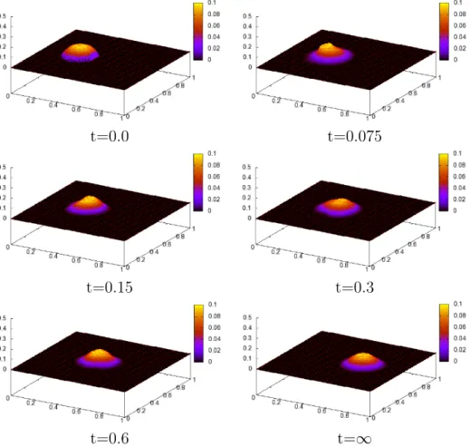
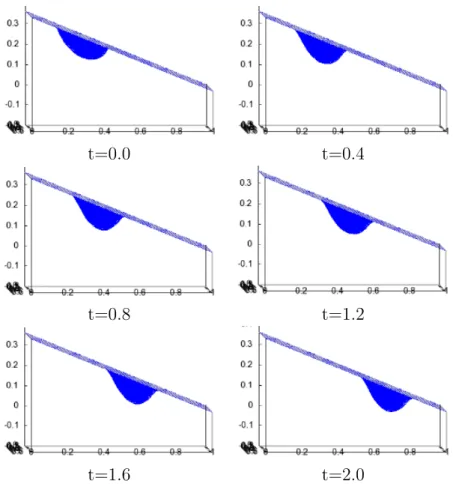
5.1 A droplet moving on plane by initial velocity. . . 36

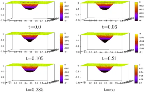
5.2 A droplet hanging on the plane. . . 37

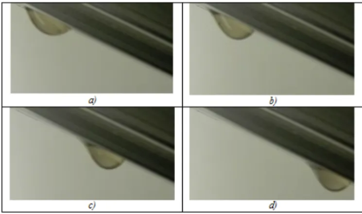
6.1 A droplet lying under inclined plane (experiment). . . 42

6.2 A droplet lying under inclined plane (simulation). . . 43

A.1 Shape function. . . 48

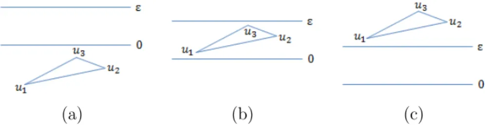
B.1 Case 1, 2 and 3. . . 50

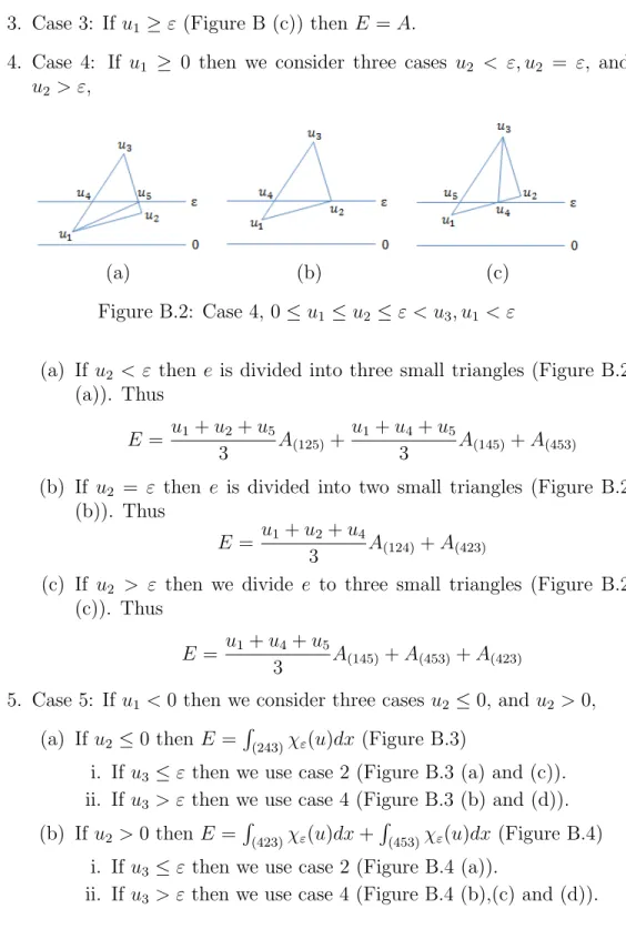
B.2 Case 4, 0≤u₁ ≤u₂ ≤ε < u₃, u₁ < ε . . . 51

B.3 Case 5, u₁ < u₂ ≤0< u₃. . . 52

B.4 Case 5, u₁ <0< u₂ < u₃. . . 52

Chapter 1 Introduction

In this study, we develop a simple model for the motion of a droplet on a plane, especially on an inclined plane. The hyperbolic free-boundary problem under the volume conservation constraint plays an important role in this model. The droplet consists of two parts: a film and liquid filling inside the film. The film must have constant volume, i.e, the volume of the region between the film and the underlying surface has to be constant in time.

Because of this point, we shall see that a complicated non-local term appears in the model equation. Furthermore, the positive contact angle is the main feature of the drop on plane. In the equilibrium case, the contact angle θ of the droplet depends on the properties of the liquid and the material on which the droplet is lying [19]. It is described by Young’s equation

γ_SG−γ_SL =γ_LGcosθ, (1.1) where γSG is the solid surface tension, γLG is the liquid surface tension, and γ_SL is the solid/liquid interfacial surface tension (Figure 1.1).

Figure 1.1: The equilibrium of droplet on plane.

In our work, θ <90⁰ is consistently considered. Therefore, the shape of film can be described as a scalar function

u: (0, T)×Ω−→r,

where (0, T) is the time interval and Ω is the domain where the motion is considered. The set where the film touches the plane is referred as the free boundary. The resulting problem for the membrane is a free boundary equa- tion with a complicated nonlocal term. We shall obtain governing equation in Chapter 2. It has the following form

χ_u>0σu_tt =γ_g∆u−ρguχ_u>0−R²χ⁰_ε(u) +λ. (1.2) This equation with initial conditions and boundary condition can be solved by the variational method, namely discrete Morse flow, which is explained in details in Chapter 3.

For fluid inside the film, we consider the fluid flow following the Euler equations

Dρ

Dt +ρ∇.v = 0, in ∪t∈(0,T)Ω_f(t)× {t}, Dv

Dt =−1

ρ∇P +g, in ∪t∈(0,T)Ω_f(t)× {t},

where v is the velocity, P is the pressure and g is the gravitation force.

These equations are solved by smooth particle hydrodynamic method. The liquid and the membrane interact in the model via pressure forces, therefore the outer force term plays an important roles in this case.

To continue this Chapter, Chapter 2 will present the model equation for the surface of the droplet, introducing the discrete Morse flow method which is described in details on the example of the hyperbolic equation in the Chapter 3. Chapter 4 represents the basic of smooth particle hydrodynamic method which uses to solve Euler equations. In Chapter 5, the discrete Morse flow is use to construct an approximation solution of the hyperbolic equation.

Chapter 6 introduces the couple model which combines the above mentioned hyperbolic equation for film and Euler equations for the fluid filling the film.

Chapter 7 draws important conclusions of the research and suggestions some recommendations for further studies.

Notations

We provide a list of notations used in the thesis

N natural numbers,

R^m m dimensional real Euclidean space (R=R¹),

Ω bounded domain in R^m with Lipschitz boundary, corresponding to the spatial region, where the equation is solved,

∂Ω boundary of domain Ω,

|Ω| the Lebesgue measure of Ω, Ω closure of the set Ω,

T a positive real value representing the final time, Q_T the open time-space cylinder (0, T)×Ω,

V a positive real value representing the volume,

κ, κ_V sets of functions from certain spaces satisfying the volume con- straint,

u unknown function,

ut partial derivative u respect to time t (= ^∂u_∂t),

∇u gradient of u with respect to spatial variables (=

(u_x1, u_x2, . . . , u_xm)),

4u the Laplace operator respect to space (= ^∂_∂x^2u2 1

+ ^∂_∂x^2u2 2

+. . .+_∂x^∂22^u m), u|_∂Ω the trace of uon ∂Ω,

u0, v0 initial data (shape and velocity, respectively),

λ Lagrange multiplier, nonlocal term originating in the volume con- straint,

h positive real value, time step of the discretization in time, a.e. means ”almost everywhere” or ”almost every”,

{u >0} set of point (t,x) from Q_T, for which u(t, x)>0,

χu>0 characteristic (or indicator) function of the set {u >0},

C denotes a generic positive constant, independent of parameters in equation,

Ωf the domain filled with fluid, v the velocity of fluid,

r the position of fluid,

n the unit outer normal vector of the membrane, g the gravitation force,

P the pressure of fluid, ρ the density of fluid,

σ the area density of membrane,

m the mass of fluid,

D

Dt material derivative = _∂t^∂ +v.∇

, W the interpolating kernel,

c the sound speed,

C(Ω) continuous functions u: Ω−→R

C^k(Ω) functions u: Ω−→R that are k-times continuously differentiable, C^∞(Ω) functions u: Ω−→R that are infinitely differentiable,

C₀^∞(Ω) functions C^∞(Ω) with compact support

L^p(Ω) functionsu: Ω−→Rthat are Lebesgue measurable andkuk_L^p_(Ω) <

∞, where kukL^p(Ω) = (R

Ω|u|^pdx)^1p,

L^∞(Ω) functions u : Ω −→ R that are Lebesgue measurable and kuk_L^∞_(Ω)<∞, wherekuk_L^∞_(Ω) =ess sup_Ω|u|,

W^k,p(Ω) locally summable functions u : Ω −→ R such that for each mul- tiindex α with |α| ≤ k, D^αu exists in weak sense and belongs to L^p(Ω). The norm is defined as follows:

kuk_W^k,p_(Ω) =

X

|α|≤k

Z

Ω

|D^αu|^pdx ¹_p

,

kuk_W^k,∞_(Ω)= X

|α|≤k

ess sup_Ω|D^αu|,

H^k(Ω) =W^k,2(Ω),

H₀¹(Ω) the closure of C₀^∞(Ω) inH¹(Ω),

L^p(0, T;X) measurable functionsu: [0, T]−→Xwithkuk_L^p_(0,T;X) <∞, where kuk_L^p_(0,T;X) = (RT

0 kuk^p_Xdt)^p1,

L^∞(0, T;X) measurable functions u : [0, T] −→ X with kuk_L^∞_(0,T;X) < ∞, where kuk_L^∞_(0,T;X) =ess sup_0≤t≤Tkuk_X,

W^1,p(0, T;X) functions u∈L^p(0, T;X) such thatu_texists in the weak sense and belongs to L^p(0, T;X). The norm is

kuk_W^1,p_(0,T;X) = Z T

0

ku(t)k^p_X +ku_t(t)k^p_Xdt ¹_p

,

W^1,∞(0, T;X) functionsu∈L^∞(0, T;X) such thatu_t exists in the weak sense and belongs to L^∞(0, T;X). The norm is

kuk_W^1,∞_(0,T;X) =ess sup_0≤t≤T(ku(t)k_X +ku_t(t)k_X),

H¹(0, T;X) =W^1,2(0, T;X),

C₀^∞(Ω;R^m) function u: Ω→R^m,with u_i ∈C₀^∞(Ω), i= 1,2, .., m,

Chapter 2

Modelling of the surface of a droplet

Modelling of the motion of a droplet consists of two stages: deriving the model of the film representing the surface of the drop and deriving the model of the fluid inside the film. In this Chapter, we focus on the film model.

2.1 A droplet on the plane

In this case, we consider a droplet on a plane. For simplicity, we assume that the area density of the surface of the drop is constant and that the surface tension is homogeneous. In addition, the contact angle of θ < 90^◦ is our consistent consideration.

Examining the equilibrium shape of the droplet is our starting point.

From the assumption of the contact angle being less than 90⁰ the surface of the droplet can be described by the graph of scalar function below

u: Ω×(0, T)−→R,

where (0, T) is the time interval and Ω ⊂ R^m(m ∈ N\ {0}) is the domain where the motion is considered. The boundary∂Ω is assumed to be Lipschitz on which Dirichlet condition is prescribed. The film is assumed not to go under the plane. Moreover, the volume preservation of the film is crucial assumption

Z

uχu>0dx=V >0.

The surface energy of the stable droplet can be written as E =

Z

Ω

γ_gp

1 +|∇u|²χ_u>0dx+ Z

Ω

γ_sχ_u>0dx (2.1)

where γ_g =γ_LG, γ_s =γ_SL−γ_SG (Figure. 1.1).

If we assume that the minimizer exists and is smooth, we obtain the following result (see [15]).

Lemma 1. Let the minimizer of (2.1) be smooth in {u >0}. Then Young’s equation

γ_s =−γ_gcosθ hold on ∂{u >0}.

Proof. We denote

u_ε =V u+εϕ V +εΦ where Φ =R

Ωϕdx. Then we have 0 = lim

ε→0

1

ε(E(u_ε)−E(u))

= lim

ε→0

γ_g ε

Z

Ω

s

1 + |∇u+ε∇ϕ|²

(1 +εΦ/V)²χuε>0−p

1 +|∇u|²χu>0

dx + lim

ε→0

1 ε

Z

Ω

γ_s(χ_uε>0−χ_u>0)dx

=γ_g Z

Ω

∇u∇ϕ−_V¹|∇u|²Φ

p1 +|∇u|² χ_u>0dx

=γg

Z

Ω

∇u∇ϕ

p1 +|∇u|² − 1 V

|∇u|² p1 +|∇u|²Φ

χu>0dx

=γ_g Z

Ω

∇u∇ϕ

p1 +|∇u|² −λϕ

χ_u>0dx, where λ= _V¹ R

Ω

|∇u|²

√

1+|∇u|²dx.

Using Green’s theorem we have following form γ_g

Z

Ω

∇. ∇u p1 +|∇u|²

+λ

ϕdx= 0, ∀ϕ∈C₀^∞(Ω∩ {u >0}) (2.2)

On the other hand, we can carry out the so-called inner variation of (2.1), which uses the perturbation

u_ε = V

V_εu(τ_ε⁻¹(x)), where

τε(x) =x+εη(x), η∈C₀^∞(Ω,R^m) with Jacobian

|Dτε|= 1 +ε(∇.η) +o(ε), ε→0,

and V_ε is determined so that the perturbation preserves volume:

V_ε= Z

Ω

u(τ_ε⁻¹(x))dx= Z

Ω

u(y)|Dτ_ε(y)|dy=V+ε Z

Ω

u(∇.η)dx+o(ε), ε→0.

Noting that if we denote

y_i(x) =x_i+εη_i(x) then

∂y_i

∂x_j(x) =δij +ε∂η_i

∂x_j(x)

∂x_j

∂y_i(y) =δ_ji−ε∂η_j

∂x_i(x) +o(ε), ε→0.

∂uε

∂y_i(y) = V V_ε

X

j

∂u

∂x_j(x)∂xj

∂y_i(y)

= V Vε

X

j

∂u

∂xj

(x)

δ_ji− ∂η_j

∂xi

(x) +o(ε)

, ε→0

= V V_ε

∂u

∂x_i(x)−εX

j

∂u

∂x_j

∂η_j

∂x_i(x)

!

+o(ε), ε→0.

= V V_ε

∂u

∂x_i(τ_ε⁻¹(y))−εX

j

∂u

∂x_j

∂ηj

∂x_i(τ_ε⁻¹(y))

!

+o(ε), ε→0.

and employing the substitution x=τ_ε⁻¹(y), we have 0 = lim

ε→0

1

ε(E(uε)−E(u))

= lim

ε→0

γ_g ε

Z

Ω

s

1 + V² V_ε²

X

i

∂u

∂x_i −εX

j

∂u

∂x_j

∂η_j

∂x_i 2

(1 +ε∇.η)−p

1 +|∇u|²

!

χu>0dx + lim

ε→0

1 ε

Z

Ω

(γ_s(τ_ε)(1 +ε∇.η)−γ_s)χ_u>0dx

= lim

ε→0

γ_g ε

Z

Ω

2ε∇.η+ ^V_V²2 ε

|∇u|²−2εP

i,j

∂u

∂xi

∂u

∂xj

∂ηj

∂xi

(1 + 2ε∇.η)− |∇u|² 2p

1 +|∇u|² χ_u>0dx

+ Z

Ω

γ_s(τ_ε)−γ_s

ε +γ_s(τ_ε)(∇.η)

!

χ_u>0dx

=γ_g Z

{u>0}

(1 +|∇u|²)(∇.η)− ∇u^TDη∇u

p(1 +|∇u|² −λu(∇.η)

! dx+

Z

{u>0}

∇.(γ_sη)dx.

Using Green’s theorem, we have Z

{u>0}

u(∇.η)dx=− Z

{u>0}

∇u.ηdx+ Z

∂{u>0}

u(η.ν)dS Z

{u>0}

∇.(γ_sη)dx=−0 + Z

∂{u>0}

γ_s(η.ν)dx Z

{u>0}

(1 +|∇u|²)(∇.η)

p(1 +|∇u|² dx=− Z

{u>0}

∇u^TD²uη p1 +|∇u|²dx+

Z

∂{u>0}

p1 +|∇u|²(η.ν)dS Z

{u>0}

∇u

p(1 +|∇u|².∇(∇u.η)dx=− Z

{u>0}

∇. ∇u

p1 +|∇u|²

!

(∇u.η)dx +

Z

∂{u>0}

(∇u.η) ∇u.ν p1 +|∇u|²

! dS On the other hand, we have

Z

{u>0}

∇u

p1 +|∇u|².∇(∇u.η)dx= Z

{u>0}

∇u^TD²uη+∇u^TDη∇u p1 +|∇u|² dx

So we obtain Z

{u>0}

∇u^TDη∇u

p1 +|∇u|²dx=− Z

{u>0}

∇u^TD²uη p1 +|∇u|²dx−

Z

{u>0}

∇. ∇u

p1 +|∇u|²

!

(∇u.η)dx

+ Z

∂{u>0}

(∇u.η) ∇u.ν p1 +|∇u|²

! dS where ν =−_|∇u|^∇u is the unit outer normal to ∂{u >0}.

From these results, we get 0 =γ_g

Z

{u>0}

"

∇. ∇u

p1 +|∇u|²

! +λ

#

(∇u.η)dx

+ Z

∂{u>0}

γ_gp

1 +|∇u|²− |∇u|² p1 +|∇u|²

+γ_s

!

(η.ν)dS, Using the result (2.2), which yields:

0 = Z

∂{u>0}

γ_gp

1 +|∇u|²− |∇u|² p1 +|∇u|²

+γ_s

!

(η.ν)dS, ∀η∈C₀^∞(Ω,R^m).

We conclude that

γs =− 1

p1 +|∇u|²γg on ∂{u >0}, On the other the hand, we have tanθ =|∇u|, which yields

γ_s=−γ_gcosθ on∂{u >0}

We rewrite equation (2.1) as follows:

E = Z

Ω

γ_gp

1 +|∇u|²dx+ Z

Ω

(γ_g+γ_s)χ_u>0dx−γ_g|Ω|. (2.3) Now suppose that the gradient of u remains small (i.e, the deformation of the film is very small) then by Taylor expansion we have

p1 +|∇u|² '1 + 1 2|∇u|²

Thus, we can write the approximation of the surface energy (2.3) in the form E˜ =

Z

Ω

γ_g

2 |∇u|²dx+ Z

Ω

R²χ_u>0dx (2.4)

where R² =γ_g +γ_s. Potential energy of fluid surrounded by the film is ρg

Z

Ω

1

2u²χu>0dx,

whereρis the fluid density. On other hand, the kinetic energy of the vertical movement of the film is given by

Z

Ω

σ

2u²_tχ_u>0 dx,

where σ is the area density of the surface. Therefore, the Lagrangian for the film can be written as

L(u, t) = Z

Ω

σ

2u²_tχ_u>0− γ_g

2 |∇u|²−R²χ_ε(u)−1

2ρgu²χ_u>0 dx,

whereχu>0 in equation (2.4) is replaced by a smoothing functionχε ∈C²(R) satisfying

χ_ε(s) =

1, if s≥ε, 0, if s≤0

and |χ⁰_ε(s)| ≤ C/ε for s ∈ (0, ε). The purpose of smoothing is to avoid the presence of delta function in the equation [15].

The equation of motion within time interval (0, T) can be defined by J(u) =

Z T 0

L(u, t)dt,

and the problem is determining the stationary point of functional J in the suitable function space satisfying the given volume constraint V >0.

Problem 1. Find the stationary state u of functional J(u) =

Z T 0

Z

Ω

σ

2u²_tχu>0− γ_g

2|∇u|²−R²χε(u)− 1

2ρgu²χu>0

dxdt,

in the function space K =n

u∈H¹(Ω_T);u|_∂Ω = 0, Z

Ω

uχ_u>0 =Vo ,

where u₀(x) is the initial shape and v₀ is the initial velocity of the film.

Let u be a stationary point of J. We select an arbitrary function ϕ ∈ C₀^∞((0, T)×(Ω∩ {u >0})), and denote

Φ(t) = Z

Ω

ϕ(t, x)dx.

u_ε= (u+εϕ) V V +εΦ. If A is denoted byA= _V+εΦ^V then we obtain

ε→0limA= 1,

ε→0limA_t = lim

ε→0

εVΦ_t

(V −εΦ)² = 0,

ε→0lim dA

dε = lim

ε→0

VΦ

(V −εΦ)² =−Φ V ,

ε→0lim d

dεA_t =−Φt

V ,

ε→0lim d

dεA² =−2Φ V ,

ε→0lim d

dε(AA_t) =−Φ_t V ,

ε→0lim d

dεA²_t = 0.

(2.5)

Thanks to above relations we can calculate the first derivative of each term

in functional J(u) :

ε→0lim d dε

Z T 0

Z

Ω

σ

2[(u_ε)_t]²χ_u>0dxdt= Z T

0

Z

Ω

σh

u_tϕ_t− 1

V u_t(u_tΦ +uΦ_t)i

χ_u>0dxdt

= Z T

0

Z

Ω

σh

−u_ttϕ− 1

V u_t(uΦ)_ti

χ_u>0dxdt

= Z T

0

Z

Ω

σh

−u_ttϕ+ 1

Vu_ttuΦi

χ_u>0dxdt, limε→0

d dε

Z T 0

Z

Ω

γ_g

2|∇u_ε|²dxdt= Z T

0

Z

Ω

γ_g

∇u∇ϕ− 1

V (∇u)²Φ dxdt

= Z T

0

Z

Ω

γ_g

−∆uϕ− 1

V (∇u)²Φ dxdt, limε→0

d dε

Z T 0

Z

Ω

R²χ_ε(u_ε)dxdt= Z T

0

Z

Ω

R²χ⁰_ε(u) ϕ− 1 V uΦ

dxdt,

ε→0lim d dε

Z T 0

Z

Ω

1

2ρgu²_εχ_u>0dxdt= Z T

0

Z

Ω

ρg uϕ− 1 V u²Φ

χ_u>0dxdt Since u is a stationary point, we have

0 = dJ(u_ε) dε

ε=0

= Z T

0

Z

Ω

−σuttχu>0+γg∆u−R²χ⁰_ε(u)−ρguχu>0

ϕdxdt + 1

V Z T

0

Z

Ω

σuuttχu>0+γg(∇u)²+R²uχ⁰_ε(u) +ρgu²χu>0

Φdxdt

= Z T

0

Z

Ω

−σuttχu>0+γg∆u−R²χ⁰_ε(u)−ρguχu>0+λ

ϕdxdt where

λ= 1 V

Z

Ω

σuuttχu>0+γg(∇u)²+R²uχ⁰_ε(u) +ρgu²χu>0

dx.

The strong version of the above formulation is as follows:

χ_u>0σu_tt =γ_g∆u−ρguχ_u>0−R²χ⁰_ε(u) +λ. (2.6)

2.2 A droplet on inclined plane

In the case of a droplet on inclined plane with angleαabove equation becomes χ_u>0σu_tt =γ_g∆u−f χ_u>0 −R²χ⁰_ε(u) +λ, (2.7) where f =ρg(ucosα−x1sinα),here x1 is the horizontal axis, and

λ = 1 V

Z

Ω

γg|∇u|²+f uχu>0+R²uχ⁰_ε(u) +σuttuχu>0

dx.

Chapter 3

Discrete Morse Flow Method

This Chapter explains Discrete Morse Flow (DMF), the variational method used in this study to solve the problem that dependent on time with dif- ferential operators for space variables in divergence form. This method was first introduced by N. Kikuchi to solve parabolic problems [1], and also used to solve hyperbolic problems [2], [5]. One of the extensions of this method was used to solve free-boundary problems [3], [4]. Solving volume-preserving problems is the other extension of this method [6], [16]. Particularly, this method can be naturally applied to the free boundary problem with volume constraint in [14], [17].

In this case, we describe the details on the example of the hyperbolic equa- tion. The content in this part is based on [15].

3.1 Mathematical formulation

We consider a bounded domain Ω⊂Rⁿwith smooth boundary∂Ω, on which homogeneous Dirichlet boundary condition is given. Then, with a fixed initial position valueu₀ ∈, H₀¹(Ω), and initial velocity v₀ ∈, H₀¹(Ω) , we consider the problem:

u_tt(t, x) = ∆u(t, x), (t, x)∈Ω_T = (0, T)×Ω, (3.1) u(t, x) = 0, (t, x)∈(0, T)×∂Ω, (3.2)

u(0, x) = u₀(x), x∈Ω, (3.3)

u_t(0, x) = v₀(x), x∈Ω. (3.4)

First, we fix a large number N >0, determine the time step h=T /N.From the initial conditions, we define u−1 using a backwards difference u−1 = u₀ −v₀h. We then define u_n ∈ H₀¹(Ω) for n = 1,2, .., N, to minimize the functional

J_n(u) :=

Z

Ω

|u−2un−1+un−2|²

2h² dx+ 1

2 Z

Ω

|∇u|²dx (3.5) In this functional, we see that the first term is continuous in L²(Ω) and the second term is lower-semicontinuous with respect to sequentially weak con- vergence in H¹(Ω). The existence of minimizers then follows immediately since the functional are bounded below for each n= 1,2, .., N.

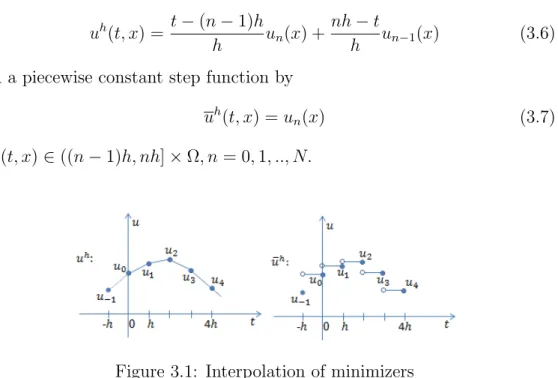
Next step, having obtained the existence of minimizers, we define their piecewise linear time interpolant by

u^h(t, x) = t−(n−1)h

h u_n(x) + nh−t

h un−1(x) (3.6) and a piecewise constant step function by

u^h(t, x) =u_n(x) (3.7)

for (t, x)∈((n−1)h, nh]×Ω, n= 0,1, .., N.

Figure 3.1: Interpolation of minimizers

Because un is a minimizer of Jn, the first variation of Jn at un vanishes.

Therefore, for any ϕ∈H₀¹(Ω) we have

0 = d

dεJ_n(u_n+εϕ)|_ε=0 = lim

ε−→0

J_n(u_n+εϕ)−J_n(u_n) ε

= lim

ε−→0

1 ε

Z

Ω

|u_n+εϕ−2un−1+un−2|²− |u_n−2un−1 +un−2|²

2h² dx

+ lim

ε−→0

1 2ε

Z

Ω

(|∇u_n+ε∇ϕ|²− |∇u_n|²)dx

= lim

ε−→0

Z

Ω

(2un+εϕ−4un−1+ 2un−2)ϕ

2h² + lim

ε−→0

1 2

Z

Ω

(2∇u_n∇ϕ+ε|∇ϕ|²)dx

= Z

Ω

u_n−2un−1+un−2

h² ϕdx+

Z

Ω

∇u_n∇ϕdx (3.8)

As we defined for u^h and u^h in equation (3.7) and (3.6) we obtain:

Z

Ω

hu^h_t(t)−u^h_t(t−h)

h ϕ+∇u^h∇ϕi

dx= 0 for a.e. t∈(h, T) ∀ϕ∈H₀¹(Ω).

(3.9) This relation satisfies with any ˜ϕ∈C([0, T]). Thus, we have:

Z T h

Z

Ω

hu^h_t(t)−u^h_t(t−h)

h ϕ+∇u^h∇ϕi

dxdt= 0 ∀ϕ∈L²(0, T;H₀¹(Ω)).

(3.10) Now, we want to take limit of time step h to zero. However, we need some more estimate. We state it in the following Lemma.

Lemma 2. Suppose Ω is a bounded domain with smooth boundary. Let J_n, n = 2,3, .., N, be the functionals defined by (3.5) and let u_n be corre- sponding minimizers in H₀¹(Ω). Define functions u^h and u^h by (3.7),(3.6) and assume h≤1. Then the following estimate holds

ku^h_t(t)k²_L2(Ω)+k∇u^h_t(t)k²_L2(Ω) ≤C_E for a.e. t ∈(0, T) (3.11) where constant C_E is defined in the proof and is independent of h.

Proof. We replace ϕin (3.8)by ϕ:=u_n−un−1. This yields Z

Ω

u_n−2un−1+un−2

h² (u_n−u_n−1)dx+ Z

Ω

(∇u_n− ∇u_n−1)∇u_ndx = 0.

Using the inequality a²

2 − b²

2 ≤(a−b)a,∀a, b∈R for two term of this, we get

Z

Ω

h un−un−1

h 2

− un−1−un−2

h

2

+|∇u_n|²− |∇un−1|²i

dx≤0 Z

Ω

h u_n−un−1

h 2

+|∇u_n|²i dx≤

Z

Ω

h un−1−un−2

h

2

+|∇un−1|²i dx.

Since these inequalities are summed from n = 1 to k≤N. Thus, we obtain Z

Ω

h u_k−uk−1

h 2

+|∇u_k|²i dx ≤

Z

Ω

h u₀−u−1

h 2

+|∇u₀|²i dx

= Z

Ω

h

(v0)²+|∇u0|²i dx

= kv₀k²_L2(Ω)+k∇u₀k²_L2(Ω).

We knowu^h_t(t) = ^uk−u_h^k−1 and∇u_k=∇u^h_t fort∈((k−1)h, kh), k = 0,1, .., N, then we get the estimate (3.11).

Thanks to the estimate(3.11), we can apply the theorem by Eberlein and Shmulyan to extract a subsequence {∇u^hk}_k∈N which converges weakly in L²(Q_T) to the function v. From the sequence {h_kl}l∈N so that {u^h_t^kl}l∈N

converges weakly in L²(Q_T) to a function U. In the sequence, we often use this logic but we shall omit this lengthy explanation and subscripts, and simply write

∇u^h_t * v in (L²(Q_T))^m, (3.12)

u^h_t * U inL²(Q_T). (3.13)

We should now show that there is a function u∈ L²(0, T;H₀¹(Ω)) such that v = ∇u and U = u_t in L²(Q_T). To this end, a more detailed analysis is needed. First, we estimate the norm of the difference of the approximate

functions u^h and u^h. Lett ∈((n−1)h, nh).Then ku^h(t)−u^h(t)k²_L2(Ω) =

Z

Ω

(u^h−u^h)²dx

= Z

Ω

u_n− t−(n−1)h

h u_n−nh−t h un−1

2

dx

= Z

Ω

nh−t h

2

(u_n−un−1)²dx

≤ Z

Ω

(u_n−u_n−1)²dx=h² Z

Ω

(u^h_t)²dx

≤ C_E²h². This means that

ku^h−u^hk_L²_(Ω) ≤Ch for a.e. t ∈(0, T).

We have further

ku^hk²_L2(QT)− ku^hk²_L2(QT) = Z T

0

Z

Ω

(((u^h)²−u^h)²)dxdt

=

N

X

n=1

Z nh (n−1)h

Z

Ω

h t−(n−1)h

h u_n− nh−t

h un−12

−u²_ni dxdt

=

N

X

n=1

Z

Ω

− 2h

3 u²_n+ h

3u_nun−1+h 3u²_n−1

dx

≤ h 6

N

X

n=1

Z

Ω

(−4u²_n+u²_n+u²_n−1+ 2u²_n−1)dx

= h

2

N

X

n=1

Z

Ω

(−u²_n+u²_n−1)dx= h 2

Z

Ω

(u²₀ −u²_N)dx

≤ h

2ku0k²_L2(Ω). In the same way we also get

k∇u^hk²_L2(QT)− k∇u^hk²_L2(QT)≤ h

2k∇u₀k²_L2(QT).

Finally, from Poincare’s inequality we know that there is a universal constant C_P so that

ku^hk_L²_(QT) ≤C_Pk∇u^hk_L²_(QT) for all h ∈(0,1). (3.14) We have obtained some results for future use. The results of the following Lemma rely only on the interpolations (3.7) and (3.6). The results are also independent of the problem under consideration and a fact frequently used later on.

Lemma 3. Let u^h and u^h be defined by (3.7) and (3.6). Then the following relations hold.

ku^h−u^hk_L²_(Ω) ≤hku^h_tk_L²_(Ω) for a.e. t∈(0, T), (3.15) ku^hk²_L2(Q_T) ≤ ku^hk²_L2(Q_T)+h

2ku0k²_L2(Ω), (3.16) k∇u^hk²_L2(QT)≤ k∇u^hk²_L2(QT)+h

2k∇u0k²_L2(Ω). (3.17) Now, (3.11), (3.17) and (3.14) imply that u^h is uniformly bounded in H¹(Q_T). Therefore, there is a weakly convergent subseguence in H¹(Q_T) and, by Rellich theorem, a strongly converging subsequence in L²(Q_T). Let us denote the cluster function as u:

u^h * uweakly inH¹(Q_T) (3.18) Because of (3.13), U = u_t holds almost everywhere. Moreover, from (3.12) for any ϕ∈C₀^∞(Q_T)

Z T 0

Z

Ω

∂u^h

∂x_i − ∂u^h

∂x_i

ϕdxdt→ Z T

0

Z

Ω

v_i− ∂u^h

∂x_i

ϕdxdt as h→0+, while at the same time

Z T 0

Z

Ω

∂u^h

∂xi

−∂u^h

∂xi

ϕdxdt=− Z T

0

Z

Ω

(u^h−u^h)∂ϕ

∂xi

dxdt→0 as h→0+, by (3.15). This means that v=∇ualmost everywhere in Q_T.

We have shown in this way that there is a function u∈H¹(Q_T), such that

∇u^h *∇u in (L²(Q_T)^m) (3.19)

u^h_t * u_t inL²(Q_T) (3.20) Now, we can pass to limit in (3.10) ash→0 +.We shall, for the time being, consider a test function ϕ belonging to C₀^∞([0, T]×Ω). To begin with, we have

h−→0lim Z T

h

Z

Ω

∇u^h∇ϕdxdt (3.21)

= lim

h−→0

Z T 0

Z

Ω

∇u^h∇ϕdxdt− lim

h−→0

Z h 0

Z

Ω

∇u^h∇ϕdxdt (3.22)

= Z T

0

Z

Ω

∇u∇ϕdxdt (3.23)

because the boundeness (3.11) of ∇u^h:

Z h 0

Z

Ω

∇u^h∇ϕdxdt ≤

Z h 0

Z

Ω

|∇u^h|²dx

1/2Z

Ω

|∇ϕ|²dx 1/2

dt

≤ Z h

0

pC_ECdt=Ch−→0. ash →0 +. Moreover, for the first part of (3.10) we have:

Z T h

Z

Ω

u^h_t(t)−u^h_t(t−h)

h ϕdxdt

= Z T

h

Z

Ω

u^h_t(t)

h ϕ(t)dxdt− Z T−h

0

Z

Ω

u^h_t(t)

h ϕ(t+h)dxdt

= Z T

0

Z

Ω

−u^h_t(t)

h (ϕ(t+h)−ϕ(t))dxdt− Z h

0

Z

Ω

u^h_t(t)

h ϕ(t)dxdt +

Z T T−h

Z

Ω

u^h_t(t)

h ϕ(t+h)dxdt (3.24)

Such that for h−→0, by using integration by part, we obtain:

h−→0lim Z T

h

Z

Ω

u^h_t(t)−u^h_t(t−h)

h ϕdxdt=

Z T 0

Z

Ω

−ut(t)ϕt(t)dxdt− Z

Ω

v0ϕ(0)dx (3.25) The convergence is deduced from the following facts:

1. in the first term of (3.24), u^h_t converges weakly and (ϕ(t)−ϕ(t+h))/h converges strongly in L²(Q_T);

2. in the second term,u^h_t = (u₁−u₀)/h=v₀ for t∈(0, h);

3. in the third term, ϕ(t+h) = 0 for t∈(T −h, T);

Finally, we get that:

Z T 0

Z

Ω

(−u_t(t)ϕ_t(t)+∇u∇ϕ)dxdt−

Z

Ω

v₀ϕ(0, x)dx= 0 ∀ϕ∈C₀^∞([0, T]×Ω) (3.26) Noting that the space of functions fromH¹(Q_T) with zero trace on ({0}×Ω)∪

([0, T]×∂Ω) is a closed linear subspace of H¹(Q_T) and, therefore, weakly closed by Mazur’s theorem, we conclude by (3.18) that u belongs to this space. Consequently, u satisfies boundary condition (3.2) and initial condi- tion (3.3) in the sense of traces. We remark that the convergence of traces follows also from the compactness of the trace operatorT :H¹(Ω) →L²(∂Ω).

Moreover, from [8] it follow that u, as a function from H¹(0, T;L²(Ω)), be- long to C([0, T];L²(Ω)). Thus, the initial condition (3.3) is satisfied even in the strong sense.

To summarize, we have proved by the discrete Morse flow method that there exist a weak solutionu∈H¹(Q_t) to problem (3.1)-(3.4) in the sense of (3.26), satisfying boundary and initial condition (3.2),(3.3) in the sense of traces.

3.2 The extensions of the DMF method

The DMF method can be naturally applied to problems with volume-constraint and free-boundary problems [15].

For hyperbolic problem with volume-constraint, we cite a result from [20]

Theorem 1. Let us consider the following hyperbolic problem:

u_tt(t, x) = ∆u(t, x) +λ(u), (t, x)∈Ω_T = (0, T)×Ω, (3.27) u(t, x) = 0, (t, x)∈(0, T)×∂Ω, (3.28)

u(0, x) = u₀(x), x∈Ω, (3.29)

u_t(0, x) = v₀(x), x∈Ω. (3.30)

where λ(u) = _V¹ R

Ω(u_ttu+|∇u|²)dx.

Let T > 0 and Ω be a bounded domain in R^m with Lipschitz continuous boundary ∂Ω. We assume thatg ∈L²(∂Ω) but put here g = 0 for simplicity.

Further u₀, v₀ belong to H¹(Ω) satisfy the compatibility conditions u₀(x) = g(x), v₀(x) = 0 for x ∈ ∂Ω and R

Ωu₀dx = V,R

Ωv₀dx = 0. Then there is a weak solutionu∈H¹(0, T;L²(Ω))∩L^∞(0, T;H₀¹(Ω)) satisfying the condition of constant volume, u(0) =u₀ and the following identity for all test function ϕ∈C₀^∞([0, T]×Ω) with Φ =R

Ωϕdx Z T

0

Z

Ω

(−u_tϕ_t+∇u∇ϕ)dxdt− Z

Ω

v₀ϕ(0)dx

= 1 V

Z T 0

Z

Ω

(−ut(uΦ)t+|∇u|²Φ)dxdt− 1 V

Z

Ω

u0v0Φ(0)dx.

For a volume-constrained free boundary hyperbolic equation in one space dimension we cite a result from [17]

Theorem 2. Let us consider the following hyperbolic problem:

χ_u>0u_tt = ∆u−f(u) +λχ_u>0(u), (t, x)∈Ω_T = (0, T)×Ω,(3.31) u(t, x) = 0, (t, x)∈(0, T)×∂Ω, (3.32)

u(0, x) = u0(x), x∈Ω, (3.33)

ut(0, x) = v0(x), x∈Ω. (3.34)

where λ(u) = _V¹ R

Ω(uttu+f(u)u+|∇u|²)dx.

Let Ω ⊂ R be a domain with Lipschitz boundary and T > 0 a given final time. Assume that f(t, x, u) is continuous in the variable u and satisfies

|f(t, x, u)| ≤Cf(u) + Γ(t, x) for some small constant Cf and a nonnegative Γ ∈ L²((0, T)×Ω). Further, assume that initial data u₀ and v₀ belong to H₀¹(Ω) satisfying the compatibility conditions R

Ωu₀dx=V,R

Ωv₀dx= 0. Then there exists a weak solution in the following sense.

A function u∈H¹(0, T;L²(Ω))∩L^∞(0, T;H₀¹(Ω)) is called a weak solution if u(0, x) =u₀, if u= 0 outside {u >0} and if the following identity holds for all ϕ(t, x)∈C₀^∞([0, T]×Ω∩ {u >0})and an arbitrary u(t, x)˜ ∈C₀^∞([0, T]× Ω∩ {u >0}) satisfying R

Ωu(t, x)dx˜ =V : Z T

0

Z

Ω

(−u_tϕ_t+∇u∇ϕ+f(u)ϕ)dxdt− Z

Ω

v₀ϕ(0)dx

= 1 V

Z T 0

Z

Ω

(−u_t(˜uΦ)_t+ (∇u∇˜u+ ˜uf(u)Φ)dxdt− 1 V

Z

Ω

˜

u₀v₀Φ(0)dx.

where Φ(t) denotes R

Ωϕ(t, x)dx and u˜₀ = ˜u(0, x).

Chapter 4

Smoothed particle

hydrodynamics method

4.1 Introduction

Smoothed particle hydrodynamics (SPH) was invented to simulate astro- physical phenomena in astrophysics. This method has been widely studied and extended for applications to problems of continuum in solid and fluid mechanics [12]. The main feature of SPH method is to replace the equations of fluid dynamics by equations for particles. In this chapter, we shall show how a continuous field can be mapped on to a series of discrete particles.

Then, we show how derivatives may be calculated.

4.2 Fundamental formulation of SPH

In order to derive the formulation of SPH, we consider two steps. The first step is the integral representation or kernel approximation of field functions.

The second one is the particle approximation.

4.2.1 Kernel approximation

To obtain kernel approximation of a (scalar) functionf(r),the trivial identity is considered the starting point

f(r) = Z

f(r⁰)δ(r−r⁰)dr⁰, (4.1)

f(r) denotes a function of position vector r, δ(r −r⁰) is the Dirac delta function, and Ω is the volume of the integral that contain r.

If we replace Delta function by a smoothing functionW(r−r⁰, h), the kernel approximation of f(r) is given by

< f(r)>=

Z

Ω

f(r⁰)W(r−r⁰, h)dr⁰. (4.2) The smoothing function W is usually chosen to be an even function. It should satisfy a number conditions, such as

The normalization condition:

Z

Ω

W(r−r⁰, h)dr⁰ = 1, (4.3) Delta function property:

h→0limW(r−r⁰, h)dr⁰ =δ(r−r⁰) (4.4) Compact condition:

W(r−r⁰, h) = 0 (4.5)

when |r −r⁰| > κh where κ is a constant related to smoothing function for point at r, and defines the effective (non-zero) area of the smoothing function. This effective area is called the support domain for the smoothing function of point r (or the support domain of that point).

Using the Taylor series expansion of f(r⁰) around r⁰, where f(r) is dif- ferentiable, we obtain following relation [12]:

< f(r)>=f(r) +O((r⁰−r)²) (4.6) Thus, the kernel approximation of a function is of second order accuracy in SPH method.

The gradient of a scalar function can be naturally calculated by taking the spatial derivative of equation (4.2):

<∇f(r)>=

Z

Ω

∇⁰f(r⁰)

W(r−r⁰, h)dr⁰. (4.7)

where ∇ and ∇⁰ are gradients with respect to r and r⁰, respectively. When we ignore the surface term, integrating by parts of (4.7) we obtain

<∇f(r)>=

Z

Ω

f(r⁰)∇W(r−r⁰, h)dr⁰. (4.8) Similarly, the kernel approximation of the derivative of a vector fieldf(r) is given by

<∇.f(r)>=

Z

Ω

f(r⁰).∇W(r−r⁰, h)dr⁰. (4.9)

4.2.2 Particle approximation

The continuous integral representations can be converted to discretized forms of summation over all the particles in the support domain. This process is carried out as follows.

At position j, we use the finite volume of the particle 4V_j to replace the infinitesimal volume dr⁰, and mass of particle at this point is given by m_j =4V_jρ_j where ρ_j is the density of particle j. Thus,

< f(r)>= Z

Ω

f(r⁰)W(r−r⁰, h)dr⁰ 'X

j

f(r_j)W(r−r_j, h)4V_j

=X

j

mj

ρ_j f(rj)W(r−rj, h) or

< f(r)>=X

j

m_j ρj

f(r_j)W(r−r_j, h) (4.10) The particle approximation for a function at particle i can finally be written as

< f(r_i)>=X

j

m_j ρj

f(r_j)W_ij (4.11)

where

W_ij =W(r_i−r_j, h)

By using the same way, the particle approximation for the spatial deriva- tive of the (scalar) function is

<∇f(r)>=X

j

m_j

ρ_j f(r_j)∇W(r−r_j, h) (4.12) To obtain higher accuracy, the particle approximation would be done by writing [9]:

ρ∇A=∇(ρA)−A∇ρ

In summary, the particle approximation for the spatial derivative of the function at particle i can finally be written as

<∇f(r_i)>= 1 ρ_i

X

j

m_j[f(r_i)−f(r_j)]∇_iW_ij (4.13) where

∇_iW_ij = r_i−r_j rij

∂W_ij

∂rij

= r_ij rij

∂W_ij

∂rij

In the case of vector field, the particle approximation for the spatial derivative at particle ican be given by:

<∇.f(r_i)>= 1 ρ_i

X

j

m_j[f(r_i)−f(r_j)].∇_iW_ij (4.14)

4.2.3 Smoothing Kernels

There are many different commonly used smoothing functions that have been implemented in SPH method. In this study we use cubic spline kernel which is defined as

W(r, h) = 1 πh³







1−1.5x²+ 0.75x³, if 0≤x <1.

0.25(2−x)³, if 1≤x≤2 0, if 2≤x

(4.15) where x= _h^r.

The gradient of the kernel is well defined for all values of x, such that

∂W(r, h)

∂r = 1

πh⁴







−3x+ 2.25x², if 0≤x <1.

−0.75(2−x)², if 1≤x≤2 0, if 2≤x

(4.16)

∇W(r, h) = r r

∂W(r, h)

∂r , r=|r|