1.7 光波測距の数値気象モデルに基づく大気補正 －浅間山への適用－

-1-

1.7 光波測距の数値気象モデルに基づく大気補正 －浅間山への適用－

 ­€

‚ƒ„­ ­…†‡ˆ‰Š

‹Œ Ž‘’“”•–—˜™

š€›œžŸ¡¢£…†¤

¥ ¦ §¨© ¥ ¦ §¨ª

£ £ £

«¬®¯ °±² ³´µ¶ ·¸ ¹

º º

, ,

AKAGI UKUI HIMBORI IJIMA

( )

Asamayama Resident O ce for Volcanic Disaster Miti- gation, JMA, , Kitakura, Nagakura, Karuizawa,

Research Division, Research and Development Bureau,

Electro-optical distance measurement (EDM) and Global positioning System (GPS) observation are applied to monitor precise time variation of the ground deformation at active volcanoes. But observations using electromagnetic waves such as these are accompanied by errors associated with inhomogeneity of refractive index along the propagation path in atmosphere. In particular, the inhomogeneity in troposphere degrades the accuracy of positioning. An improved atmospheric correction method in EDM was developed, based on the Japan Meteorological Agency (JMA) operational mesoscale analysis (MANAL) for numerical weather predic- tion. In this method, the precise velocity and ray path of propagated lights are estimated from the adequate vertical profile of refractive index by MANAL. Consequently distance along the bowing ray path measured by EDM is corrected to be precise slope distance. Applying this procedure to EDM data at Asamayama volcano, the seasonal fluctuation caused by inhomogeneity of refractive index in atmosphere was removed entirely.

At Asamayama volcano, very small eruptions occurred in August since the latest eruption, and then a small eruption occurred in February . Based on the EDM observation by Meteorological Research Institute and Karuizawa Weather Station, we detected that the slope distance had been shortened since August . Slope distances from the observation site to reflectors were corrected by using MANAL in this correction method. Though slope distances have increased in length at a rate of mm per year since the eruptions, ground deformation turned over to inflation in August and slope distances shortened to mm per five months by January .

In order to account for those observation data, we assumed a pressure source beneath the summit crater, whose depth and volume increase were estimated to be at a height of m above sea level ( m under the summit) and , m , respectively.

By developing this atmospheric correction method in EDM with the use of the JMA’s numerical weather model, it became possible to precisely detect ground displacements and thus to reliably estimate their sources.

Therefore, this method is very e ective to monitor activity of volcanoes.

: Atmospheric Correction, EDM, JMA numerical weather model, Asamayama volcano, MANAL

Technology - Japan.

Seismology and Volcanology Research Department, Meteorological Research Institute, Nagamine, Tsukuba, Ibaraki, Japan.

:

Nagano, , Japan.

Present address : Earthquake and Disaster-Reduction

Corresponding author : Akimichi Takagi Ministry of Education, Culture, Sports, Science and e-mail : [email protected]

Akimichi T , Keiichi F , Toshiki S and Sei I

Atmospheric Correction in EDM by Using the JMA Numerical Weather Model : Application to Measurement at Asamayama Volcano

Key words

-

// ,*+*

+ .+ /+

$ +1*0 2

,**3 2 -+ ,*+* + +/

,**2 ,**.

,**3 ,**2

+ 1 ,**.

,**2 / ,2

,**3

,-2* ,**

+/ -**

#

-*/ **/, + +

-23 *+++

+1*0 2 + +

-*/ **/,

+** 23/3 - , ,

-23 *+++

   

  ­€  

‚ ƒ„ … †‡ˆ ‰ Š

‹ Œ Ž‡ Œ ‘’“ ”’ • …–—‚ ˜ ™— š› œžŸ¡¢… †‡ £ …™¤ • ¥†‡ Ž‡ ¦§¨

‘‚©  ª«¬Ž ®¯‚°±Ž¤   …­¯†²‡

™¤© „ ³ ‘©Ž‡ ‘ ‹ ‰  ´µ ¶

’­© · ‚ Ž€­¸ˆ ·¹ º»¼½¾Œ ‘— ­€‚­¯ ’—‘

¼¿À ’Á¯ ´ ¶º»¼½¾³ ‡

Ž‡ ÂÃÄÅÁ‚ µ µ Æ©  … †‡ˆ  ¶Ç¢‚ÈÉ Ã ­€Ê …• ’€ ‡‘­€ Ë ‘‘©™¤ Ì ¤ ÍΒ

”’ÏЩÑÁ Ò Œ Ž‡ ‡  ‚ ƒÃ µ Ó

Ô ÇÕ» ’ Ö׃Ø

Ù ‚ ’Ú‡ Û ·  ÇÕ»… ’ … ‹ ܅’ Ý ‘Þ œ ß­€ „ … œ ’­’ à™¤© Ì  ÇÕ»

†‡ ‘á †‡ ’âã‚–Æ àä ‚  

£  ‘ Ž‡‚ ‚ ¦ Ì Ú‡¶Ç¢  ÇÕ»…

ΐ ‘€ £ ‚ åæ ç è £ …Èɒ ’éê ë †‡ àˆ ìå… ’ • ‰ âㅖ ÏíÁ¯‡ ™¤

„ …É݆‡ˆ‚ ¦ Î†î  Ü†‡ ¼ï¢»ðÀ …–—ˆ

í … †‡‘ ’ Ïñ‚ò Ž ‘‡ … ©à …â

‡ àˆ  ‚óô õö Ž‡‚óô ã’

‘ · õö ÇÕ»… ’ ¦ €Œ … ƒÃÁ¯‡ ÇÕ» †

‘’ ‡‘ ÷¬ … ‡‘ „ øù ’ú û Œ ‘üý µ þÿà ~}’ µ ÿ‚ †‡‘

‘á Âà |Á¯‡ ‚óô ‘ · …â݆‡‘

ß ‘ Ž‡‚µ ÂÂÊ

• ­€ ‘‡‘ é

ê õö®¯ ’ ÇÕ»™‡   ‚   { ˆ [

‚ •„ É݂ \ Ž‡ …] ’‡ ˆ ¶Ç¢‚

^ … |‘†‡ ^¶Ç¢ ^¶Ç¢

_`… @± ‘’ Û …™¤?­ †

‚ ˜ > …‹ † ‡=<¶Ç¢ ¶Ç¢Ž¤ Ï{;

‡ˆ¨… :’ Š à ‚ ‡ /ÏÐ .¶Ç¢ ÍÖ× ƒØ

@± æ> ­€ ¤ Ó ‚ ^¶Ç¢ =<¶Ç¢‚ Ž‡  -© ‡‘ ܒ ñ ÇÕ»­€£ > ÍÖ× ƒØ‚ ‚ ˜,

> ¹+*)𢅠€­†‡ˆ ( '½Ç & Î ,& ¶Ç¢ % … ’‡

  

  ­€ ‚ ƒ„

…†

‡ˆ ‰ ‡ˆ Š

‹ Œ† ƒ„ ‹ Ž

‘’ Š

‰ Š “ ” • – —˜

™ š › œž ­ ‰ –Ÿ‡ˆ

 ¡ ¢£ ¤ Š¥

¦ § ¨© —

ª « ¬— — ˜ Ž® ¯ Ÿ

° ¯ ‡ˆ ­ ‰ —˜ §

±² ³ ´

  µ ±²¶ˆ · ±² ­ ‰ —˜ ®

¸   ¹   º®

ˆ » ¼ º½

±² ¸ Ÿ

¾ ¿ À ƒ„ –Ÿ˜ ® ‡ˆ

Á

‹  š ¸ à £ º®

˜ ® Ä Å Æ

Ç ŠÈ ÉÊ Š ËÌ

‹

Í Š š

› Î ·

´ Ï –Ÿ Ð —˜–Ÿ

¼ ­ Ñ Ò —˜–Ÿ

šÓ –ŸÔ š š –

Ÿ ÕÖ ˜ Ï× Ø –Ÿ

Ö Ù­€ Ú Û –Ÿ ®

Ü Ý ¢ ¨©”

Ù­€ Ï Þ ¥ š

‡ˆ Ÿ   ” ٔ 

Ù ß à á â Ö ã ¡

( ) Fujii and Miyamoto 42

;

GPS

GPS

GPS

( )

km

mm

S N

( )

( )

km km

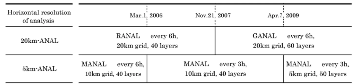
Table . History of two ANALs’ horizontal resolution used to this atmospheric correction.

+31*

, +31* +320

-

,**/ ,**.

,**- ,*

+33.

+ ,

+321

+32+ ,**3 2

,* /

+ +

,



 

 

  

 

 

 

 



   

   

 



 

  

  

 









  

 

   

 ­€‚ƒ„…†‡ˆ‰­Š‹

ŒŽ‘‹’“”•€–—˜†“™†„†

š‹ › œžŸ¡ ¢£¤¥¦

§ ¨©ª«¬® €¯°±²¬ ³ ´µ¶·

¸ Ÿ …„ † ¹º»¼

½¾ ˜¿À€Á ÃÄņ‹ ¹ …„ ¼ ¹ †Â Æ Æ ÇÈ ÉÊ ª« ËÌÍ ÎÁ̀ Ÿ ÉÏÐÑ Ò‹ Ó

€ ÔÕÖ× ‹ ÔÕÖ×ØÙ²¬ § ¨©²¬ ³€Ú œžŸ¡«

¢£ ۚ

⬌Ž Ü݀ Þ߁¢£¤à ¢£ ۚ ’ áâ

”•€ã͋ä圞Ÿ¡ ²¬æ¹€ç— ¢£ è é Ÿ ˜ êϹëÚ ÔÕÖ׆‹¢£¤¥¦äŠ ìíÌ îï €ðš ⁠ñ

´µò €ó“‹¸ ¢£¤ €ðš

ۚ ³€  Ÿ¡ô áõ

Ó Ÿ ņ‹ª« €‚š‹

€Á‹ § ¨©²¬ ³€·

³ö÷ øš‹ · š‹¨©¥¦ á ‹ ⁠²¬ ³ù ñ …„ á⋠ÎÕú€ª«¬® ¨©ôûü¤ýþ€‚ é ÿ Ë~ó ñ é ݀}­|{« 

Ÿ ˜þ‹ ²‘† [ á ⸠¢£ÇÈ

¢£ \ ]^ ¢£Ê ဴµµ_`@?…„ >

=µ>? <À € ;£ :¤

á õ /ß ¢£ .- › ,€ á€

+ † â ½*¸ € á€`@?>)€ .

Ÿ €†Â â á …„ - :¤Ç ( ž¨ '&%

 





 

km-ANAL UTC

km-ANAL km-ANAL UTC

(MANAL)

ANAL GPV

43

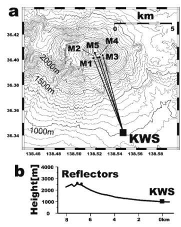
Fig. . Distribution of horizontal grid points of every ANALs around Asamayama volcano. Squares,

circles and diamonds denote km-RANAL, Fig. . Distribution of reflector sites (M -M ) and km-MANAL and km-MANAL, respectively. observation site (a), and topographical profile (b).

km km

km ANAL km-ANAL km

ANAL km-ANAL

km GPV

Table ANAL

Fig.

GPV

ANAL GPV

ANAL GPV

ANAL GPV

km (GANAL)

km (RANAL) km m

(M , M , M )

RANAL GANAL (Fig. ) M

km RANAL M M M

MANAL GPS

/ ** -

/ ,* **

- ,**1 ++

+

,* +* , + /

/

+* /

,**3

,* ,* /

/ ,**3 -

+* ,

+

+ ,**0 -

,**- / 0

,**3 1

,**1 ++

,* 0* ,*

+* ,**, 1 /**

- + , - -

,+ , ,**/ 2 ,

,* - . ,**/ 3 /

,**3 . 1

-



   ­ €‚ƒ„ …

† ‡ ˆ‰Š ‹ Œ Ž

‘’“”• –—˜™š › œž Ÿ¡ ¢ £ ¤Š 

¥¦§¥ ¨©ª«¬®¯ °±² ¤

³´µ ¶· ¸ˆ¹º» ¼½¾¿À

º» …ÁÂÁ Ä ¢ ¨ÅƝœž ¤Š „ ÇÈ ÉÊË…ÌÍÎ ½Ï¡ œžÐ ¤ÑÒÓ ½Ô¢

¦ÕÔ Öµ †

Ó ¢ £  ¢ Ð  ¤ ×Ø

 ٝÕÔ  ÔÚÛÜÝ ÞŸÈ„ 

›  ÇßÆàáâãäå¨ Æàáâã

¸æ¨ ÅƝœž ç¡ èé ê ­ ¦ëì íî Õ¾

ïðîñ Ë  ¡ ÌÍÚ» ò ¦

ó Ï¡ „ ³´µô õö÷„£ ÅƝœž ÷øù„£

Ç ¥¦³´µ €úûü  È ýӝþÿ

¦È –~ ӝ„ ½¡

Ó}’|{[\ ýÓ]ÓÏ¡ }’| ®

^­ }’|äå¨

…_ `¨  ¦ Äӝ ÅƝœž ¤ ¢ µ Í ³´µ Öµ™@? `¨ Ð >ØÅƝœž ¤=ÓÞ „£

¦µ©Í`¨ ¤<È ©ªÈ õö÷œž

¡ ‚ÅÆ † Æ; Æ:

Çß/€„œž

„¢ £ ÅƝœž ½Ô ¼¨ ½Ô

³´µ Öµª.²©Í¤ Ô ¢ Š ™µœž -,ÅÆ+*Æ Ð >ÅÆ)(Ë ² ö ² '&¤ÚÛ ½% ½¡



 







  ­

€ ‚

ƒ

„ …

†

. km

Leica Geo- 44

Table . Specifications of electro-optical distance meters.

Table . Location of reflector sites and observation site for EDM at Asamayama volcano.

M GPS

km (KWS)

. km

Geodi- meter

systems TPS

KWS . m

M

( )

Table Fig.

Table

. km

. hPa .

C, n

v n C

v

n v

n

+ / ,**- / ,**3

,

,

-

. ,**0 /

2

1 1 /

1 .-0

0*** ,**/ - ,**1 ,

+,**

+

. ,

,

+

, ,

-

+ * * +/

+*+- ,/ + ***-

. +

.



  ­ €‚ƒ„ … †‡ˆ‰

Š „‹†ŒŽ­ ‘’“  ”•

– —˜Š™š›œžŸ¡¢ ‘ £¤¥¦§

” ¨ 

©ª ” « 

¬®¯°˜© ±² «¬®„ ¯³´

µŽ ¶ ·

– —¢ ‘   ‡Ž

¸¹ º» ¨„¼ ½

¾¿­

„ Ž­

”¯ ¬®¯°˜ ÀÁ

”   ¢ €±² ©

„ Ž‡Âǎ

‘Ä “ ³ Å

Âí„ÆÇȝ† É  ÊË̄† ÍΜ ϏžŸ¾ ÐÑ

±² „ „ Ž‡Òˆ† Ó ÊÔÕ Ö “ ³ „ȝ†­ ח„ØÙ­£¤

ڄÛÜ­ ݊„Þ †­ ¥ß àᔠâ ɋ ¤

š›œ ʮ㯠ä

¼  – —â‰¯– «  “ ³ ±² å„ æ ç ‡Žè “  éÚꪊÓë¢ ‘ ìí ȝ†­ë© ­

„ ”†•Žî ï冗ñ €‚ ò† ó ôõ†‡Ž

ƒ™Š  ‡Ž •À àᔠâö ÷¤„ø†‡ñ”†

ìí ‘ „ ‡¸¹†­ —Г ³ „ùúÁهû•

Ž‡ˆ‰†­“ ³ Å¢±² ݊” — •¨ì™üý҈†­þÿ ³ ±~Áه

}| {[¢ë ©Ù­ \

†­±² ‹„ “  éÚꪊ]|­Š ^© ¶ _`@ ?Áه â ?†

“  ‘Š”•ª җ†­“  éÚêª ­”†‡ëñ¸¹Á>‹ =Æ©ª

<¾ ©”„;í

±² Ý:•¢ Áه– “ ³ =ÅÄ „ Ž ‘î /¯“ .^

±²¯­Ã “ ³ /¯ ‘ë © ‘”“ ³ ‘-ÿ„ „ Ž‡Òˆ†‡

ӓ ³ ,¢‚ƒ„¸¹+ µÊ î *”†‡ )†­ ™

”_† àá (Å š›œ ùú *ë­¯“ .^ *'& %÷



 

 

  

­ €  €  

· ·

. .

( ) Tetens ( )

ANAL GPV

GPV are ppm and . ppm, respectively (b).

( ) ( )

atmosphere (a). Seasonal changes’ ratios of veloc- 45

( )

(hPa)

(hPa) (K) ( m)

Ciddor, ; Hill

Barrell and Sears ( )

( )

. (K) . (hPa)

. . . ( )

. . ( )

Fig. . Velocity and ray path e ect on slope distance caused by inhomogeneity of refractive index along the propagation path in atmosphere. Ray path is bended propagating through the inhomogeneous

. ( ) ity and path e ect calculated by actual JMA’s

ANAL GPV

( )

( ) ( ) (Fig. a)

. km

Fig. a KWS M

UTC

MANAL GPV

(Table )

ANAL GPV ( ) ( )

ppm

m

. mm

GPV

(Fig. b)

(KWS) ANAL

d

d w

d w

d g

w

g

Td Td

e T

p e

n m m

T T

p e

T m m

et al.,

p p e p

n n n

T T T T

T p

n n

n n

n

n

e

0 + ,

+ ,

* *

0

* *

* *

0

, .

,

1 / ,-1 -

+3-*

+/ * /

- /

+ +* ,

+330 +32*

+3-3 +33.

+ +* -

,1- +/ +*+- ,/

+ +*

,21 0+// . 2200* * *02** .

.1 .,. * /+02 /

- #

0 ++ +* 0 #

0

- / -

+ /

++ - +

,**/ +* ,* *0

,***

,

- /

-

+

* **-

- . ,

. - . .

l l

l m

l

l l

l

 ­€‚ƒ„…† ‡ ˆ‰

„Š  ‹ŒŽ ­Ž ‚ ‹ŒŽ

‘ ’ „  ‚ƒ“” •–Ž—˜™

„— ” š› œ žŸ¡¢£ 

‡ ˜ — ž¤€ ‚ƒ¥ ”

¦£§¨ © ª «

‚ —˜™¬ ­ ®¯ ˆ‰ †°

±€ †°²“­¤«Ž ³

´µ¥ € ¶ ·¸¦£§

¨ © ªŽ ’ ·¸

Œ © ¹ª – º» ®

²¼  ­€

½ —˜¾¿À ž ½ Œ

¢£ ÁÂà —˜¾¿À ė

€ Œ ´ —˜¾¿À €

ÅÆ Ç†° ǖ Ɲ È É­

”Ê€„ ËÆ ÌÍÎÏÍЗ ¢£ª Ñ Ò ƒÓ˜ ¼ ‚°ÔÕ ‚Æ ÖÆ×Ø Ù † ª

‚Æ ÚÛ ƒ Ò Š Ü ªƒ

” ƒ Ý „Þߝ…¤€ ƒ”¡ Ә à ½ ËÆ á €„ â ãä ® ² å€æª ž†ž çÅ èé êŽ ž—˜¾¿À

ë º ƒ º „Ø ªŽ ‘ —˜ ž ž ìÆ á í Œ

¤ îçÅ „­¤€€ïð ҝ à ¢£ñ€ ò”  †° êŽ

ëó çô  à ºõö÷ ª €§¨ñ ž—˜¾¿À ” ƒ

€Œ ºõö÷„øù” ú‚ „ î Œ ¢£“” òœ ïðƒ

Â…¤€ †ûÆü ƒž¤ ‚Æ ý ½ ª ÚÛ þ—çž¿À ž Ý ÿӘ Ë~ ® ² € ‚ƒ” ¢£¼“”

® ²„ ­€}û çÅ „ îÂ|¤€ ‚ ý ½ ƒ È Œ ¢

ƒ¥ ” £ „ ºõö÷¼ ºõö÷¼ ­€‚ƒ„…†

 ÚÛ †° Ò — ˜  ÖÆ× Ç Ç ãä „ª €¤ ½ Ý ž ‚Æ ý ½ ¼—{„ ã[„ ” ‚ Ә Ë~ “” òœ ïðƒ ƒ¥ ” ž¤€ ‚ƒ„…† „ ý ½ ý ½ ª ÚÛ þ—çž¿À ž õö÷„ €œ Á\ ª ž

¢£¼“” ] ^_ š ` ½  †ž ½ „ª‚ƒ„

Œ¤@?­Ó˜ ‚Æ > ” ® …† – Ç ã†°=–ä

² ª ý ½ Œ ç çÅõ –Ž ǝ  ã¼°ž„ ‚ ö÷ º „<;ž¤«Ž ú܊ ï Æ¼Ó˜ „ª ž†žý ½ ðƒ 愪 ‚‚ƒý ½ „çÅ õö÷ ¼: ” ‚ƒ”° / ª –

§¨ ë ž¤. ž¤€ ‚ƒ“” ÔՄ

½ Œ çÅõö÷ º -œ¤ ­€ „ Á\ ªŽ ý ½ ƒ Ȥ¼ú

® ² ºçÅ ,+” õö÷© }û*)ž¤€€‚ƒ„…†

ƒ(|¤Œ ºõö÷© å€ –

Ә ³ ½ Œ¤ý ½ ƒ « ‚Æ š '¾& %

 

 



  

­ €‚ ƒ ­

 „ …

‚

† †  † 

‡ ˆ ‰  Š

‹ Œ

‰ ˆ ‰ Ž ‘

’ ƒ ­  “ ” •

 † – —

˜ † ‹ €‚  “

€ ˜ ™ ˜ š

› ™ —

† € š œ

ž ­ ‰ ‚

’ Ÿ  ‚

 € ž ­ š

 †

‰ ˆ ‰ † •

‚ ƒ ­ ’ ž ­ ¡¢

Ÿ š œ ž ­

ž ­ ‰ ‚ „ £

¤ ¥ ­ ƒ ­ 

¦ † §•

 ž ­ † •

† œ ž ­

¨– ž ­ © ª ‘ “



ƒ ­ † „ £ ž ­ š

 

†

 ƒ ­ ž ­ š

cm 46

( ) ( )

ppm

ppm

. ppm

Fig. . Slope distance from KWS to M measured with auto EDM system from March, to February, . Distance corrected with MANAL has smaller seasonal noise than that by the conventional correc- tion. Parenthetic figures show standard deviation (mm).

TPS

cm M

ANAL GPV

Fig. KWS M

km-ANAL km-ANAL

km-ANAL, km-ANAL

Fig. KWS M

MANAL ( km-ANAL)

cm

(mm)

km-ANAL

. mm km-ANAL

km-ANAL n

v

ANAL

+

- +

+/

+ ,2/

* / + +*

. +

,**/

,**1

+,**

,**/ - ,**1 , , +*

+ +

,

* ,**- ,**3

/ ,

,* /

,* /

. + ,**. 3 +,

/

, ,**2 2 ,**3 ,

,*

1 . /

*

,*

/ / +

/ ,



  ­€‚ƒ„…†‡€ ˆ‰Š‹

ŒŽ‘ ’“”• ƒ –—˜™š ŒŽ

›œžŸ­ ¡ ¢£¤ƒ ¥ ¦§¨ƒ€‚Œ 

Œ ’ƒ¢©Œ ª«© ¬® ¯°ƒ¦ «©¡†¨  ±²¬ƒ

œžŸ­ Œ ³´ ° µ¶·¸” ¹š¢°•º»”Ž‘

¼ ½©“” ƒ¾¿ÀÁ‘ ¢£¤ƒ‡ ³ ˆ‰”ž«©ÂН±ƒÄ

€ ƒ ¡ ­€‚ƒ ŌÆÇ¢°ƒ£

¼ ƒÈÉŒÊ¡Ë ÌŒŽ ÍÎÏÐр‚±” Ò¤Ó Ô ° Õ Ö ×Ö •Ø´¿Œ‡¿ كڡÛ܌ݴ© Þߔ•

¡Œ ½©Œ Ń£Ë ̲¬ƒ• à Œ£¼ÚÛ܃ ”¿¢°ŒÁ³‘

š¢°•”¿á â֘㡆ä唎

° æç ±µèéêë ìí îï

ƒ£Ð‘Œ ’×ð• ×ñ³´ ƒ£‡€ •Ó Ô °µèéêëƒ ° Õ ´³ƒ¦§«©Ô ”Ž¢°ò ó ôÒ õ õ ×ð ö÷øƒ ù¢°Œ ´³ƒ‘ ³ú‰óö

ƒ£ û ŒÁá³üýþ¼ ÿ±~}|¨ ޥك~{±[딢

¡£¤ƒ\] ˆ‰• ’^“” Ô ¡ƒ• Œ_`@ݔ¿ ŒŽ

¯†î? úþ¼ >¼ ¢û üý ³ • ±=<;Œ ”¿“”ƒ 

Œú‰óöƒÄ:š³ ½©°€‚ `³³” ~{±[ë÷ø¨ƒ•½©×/

Ń£.[-, 蔎³ +š „ƒ*)«© ­ ×( °

ƒ• '†° ×ñÂÃÁ‘± š &%Ý¡





   

 

ANAL

ANAL km

47

Fig. . Slope distance corrected with km-ANAL and km-ANAL from KWS to M measured with manual EDM from to . Triangles and arrows show the eruptions at Asamayama.

RANAL km

GANAL

km km

RANAL

km-ANAL km-ANAL

km-

ANAL km

km- ANAL

GPV ANAL

ANAL FCST

,

+*

/ ,* /

, ,**- ,**3

,**1 +*

,*

,**1 ++

0* ,*

,**1

,* /

/

.

,**, ,**3 .

/

,**3 ,**3 /

,**3 /

+

0

 

  ­€‚

ƒ „… „

 †‡ˆ­‰ 

Š ‹ ŒŽ‘ ’ “ ”

• – —˜ ™ š›œ•

ž —Ÿ¡• ¢ƒ £¤¥¦§¨©ª ­«¬

®©ª ¯ž°ƒ±

² ­— „­Š³´¥¨µ¶·

¸ Œ ¹º »¼ ½š—¾

 ¿ƒ „ÀÁ    —

¸  ¿­ —

™ÂÃÄ«‰Å† Æ ƒ ÇÈ ÃÉÊ Ę̈Í΁ÏÐчÒ

­‰ ¿±² ±²Ó ч

 ¿ÀÁ   — Ԇ‡Õº

ց  ×ØÙÚ

ƒÛˆ‡Ò­ ‡ ܏ ¿ƒÀ Á    ە ݃ ƒÔƒ

Ü ƒ ¿ÀÁ ­ · Þ —

† ß©àá ܏âã ¿± ‚­Ûԏ ‡— ³´¥¨­ ‡

² ܏âã ¿±² ¯ Ÿ ƒäڍ Ù偗

ªæç ªÁÃÉʁ 脗 Ü ƒ•Û ‹ ­ ¿é  ê ꁍ •« ‡   냐

 ˜ÑÑ ¾ ¿ ìÑí · •« êÙ¶ î„ à ŠÛ•

­ ¿­‰ ­€ ž° · 

ÀÁ    ë· ïðñ ò ó 

    냐— ê ê„ ¿ÀÁ ô

    ë· õ ¯ ö„÷ø ªÁÃÉÊ­ Ü ƒ

ƒ ù…   ˜Ñ ¿ƒ£ªæÀÁ „ Ë ­ë·

¡Ô •« „ — „ ­ ö„÷ú÷Æ Š… êԈ ˜ ÏÐч«û ¿­—„ ­æñ üƒÜ ƒ ú ê ý·ù ê

  Ôê­ £ÀÁ — ­ þƒ €û

Ç­ —•Û Ü ƒ ¿ÀÁ ÷ ·ÿ~ ëƒ † — 

÷ ­} ×Ø Û ú|{­ Ë

· ™ÂÃÄ­‰ — [ þ — „ÀÁ Ë æ}\ƒ]Ò Ë^ Ԉ½šƒ ê  ¿ƒÀÁ Õ_— —`Å­ ƒÿ~‚ †‡

   ó ­ ñëƒ ñ— Õ@— ƒ •« — ? >­‰û ·  ¿è½Ñ‡ÀÁ êª …­=ª<;ƒ :Æ

   ëƒ / ñ— · „ Æ ƒ©ªÑ‡ ? — .  Ë ¯·

  „ :„ Ë — Æ 

­— ­    ەÿ~ ù[ úÆ ê ê - ƒ ÿ~— Ü ƒ±²  …Ôˆ ,ۘ+ • ú„= ­ ýƒ:[

ªÁÃÉÊ *—  Û)•ˆ• Æ ê ê ­  ('— ­ˆ‡ †‡— – Æ &%ƒ †„ÀÁ Ë ‚

 

 

 

  ­

€

‚ ƒ

 „

… †

‡ ˆ ‰   Š

‰  

‹ ‰  Š

Œ   Ž

‘ ’

‰

‰ “

‡ 



‡ ‰

”  • ‰ – — ‰ ˜™ š

 ›œ žŸ ¡

›  ¡

 – š ¡  ¢

 ‰

 £¤

’ ¥ ¦ ¥ §¨ £ ©

‰ ­ ‡

¥ ‰ ‡ ª £

 ¡

 ¡ ‰ ‡ «€

  • ‡ ‰ ¬

   ¢ ® • —

¯ … ‡ ‰ ‰ °

‡ 

FCST

UTC FCST UTC

ANAL. Open diamonds and solid diamonds show

RANAL

UTC

UTC FCST 48

(FCST) FCST

RANAL (FCST)

ANAL

FCST UTC

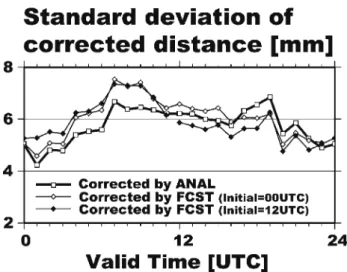
Fig. . Standard deviation of corrected distance.

Open squares show S.D. of distance corrected by ANAL

FCST that by FCST of UTC and UTC initial time,

respectively.

FCST

(ANAL) GPV

FCST

KWS-M ANAL FCST

Fig. km-ANAL (RANAL) km-ANAL

UTC mm

UTC

mm km-ANAL

UTC ( UTC) Fig.

km-ANAL

ANAL FCST mm

M

FCST UTC

FCST GPV M

UTC M

FCST

UTC M

M

UTC FCST (

UTC)

ANAL

GPV

** +,

+, ,. +

**

,**0

.

+, ,.

0

** +,

+ ,**0

. ,**0 +,

,**3 2 /

0 ,*

**

/ ,**0 .

,**0 +, **

/ /

** ,. 1

,* 0 ,**2 3

,**3 , , ,**3 +

/

0 ,2 /

+ , **

,**3 , /

** -

,**2 .

+, ,**.

+ , ,

+, *1 +3 ,**.

,**. 3 +,

,**2 2 ,**3 / 1

1 +

 ­€‚ƒ„…†‡ ˆ‰Š‹ŒŽ

‘’“”•–‘—˜™š›œž Ÿ¡ ¢ ¡£ ¤

˜–—¢ ¥¦Š§¨˜©ª«¬®¯ °±²±•³´›µ¶· ¸¹º»¼Š

ž½¾²¿²‰¼ÀÁÂÃÄÅ´ “ Ƴ´›ˆœÇ¶ÈÉ Ê˒ ¸ž “

”ÌÍΞ ˜ÏŜ ¸žÐ“” ”ÑÒϹº» Ó£ ­€

Ô՛ÊÕ Ö×عº»ÙÚ

¢ ¦ °±² Û܊§Ö× ÝÕ “”¿ ¹º»—Þߏàáâ

œ ˜ã•…Ï—¢ ½¾²Š§¨ äå˜ãæ ÅǶ Æç èËé¬

©ªê¼ ëìíïð—Þ¼ñòÏ ‰ó Æç ‰óôõ ¹º»

‘ ¦ †‡• ö÷¼ñòÏ ãŒ øù“”¿ ߏΠ“

›œÅ—¢ žž ¼ Ƈ˜ ”úû¼ Ùüýþ€ÿ~Âé¬}|

{[\]^ž à _` Ÿ¡ Š§Ø@ ¹

º» Æç?>˜’=¿ã•Ã

<Ö°±²“”¼ „ÑҞ ˜Ï žè˼;:Ö×/ Û.

°±²Ã•…Ï—¢ ž-²¼ ,³´›ˆ¨ Ûܽ¾²É+ ¥ÀÁ ÂÀÁÂ*¿ ÊÕ)ᕅϜ (– ÂÛ-¿˜Ë’ ' '“

’˜ Տã•Ã„ÑÒϹº»¼Ö×Ø ”™ù—Þ¹º»&´ žÈ °±²&¦¢

.

49

Fig. . Temporal change of slope distance corrected with km-ANAL and distribution of reflectors on and around the summit.

m

(Mogi, )

. mm year

M m

m Fig. b

km-ANAL M

km-ANAL

m m

, m

M M M

-

-

+ + /

1 /

,,** ,**/ ,**2 ,**3

+3/2 1 1

/ +*

+** 2

,* /

/

,-2* ,**

+/ -**

,**. ,**2 ,**3

+ , - - /

,**/ 3 ,**2 . 1 ,



  ­ €‚ƒ „ … †

‡ˆ‰Š ‹ŒŽ   ‘’ “” • – • —

˜™š›œžŸ ¡ ¢£¤¥ ¦ •§ ¨©ª«¬‘®¯°±²

³‘ ‘´ µ¶· ‘ ‹‡ˆ • ¸ ‘ —¹º » ‘

›¼ ½  —•¾¿ ÀÁ — Â۝‡Äŋ

Æ œ¢Ç ÈÉÈʵ Ë ‘žÌ¡›– ‘ ÍÁÎÏÐ

ÑÒ̜  ÓÒ̜ Ô£ Ց´ ։Š×Ø¡

µ’ ÙÚ Û‘Ü ³Ý Þ Žœ

ßà  ‘‡ˆ —¦ • Æ ¤• ¿á¿ÍÇ

¯Žœ ‘á¿ âã ̐Žœ

‘äˆ ͒ ‘ååŒ ‘´ µ

‘Ç æçèéꍛ  ¤ëì

• ̐· Œ ‘ÈÉÈÇ  ÈÉ ‘– ¯Ô í€îïˆ º ÈʵÑÒ¨¶· ‘’ •ðºñ ¤ ò ó ˆ‘ôõáà Íö •

©÷øÖù•° ÍñœžÍÌÍ  ‘ ¾œ à úûü ýþ ÿü ~ß ü

•Í}‡ˆ•´ µ | ¯Žœ £ñ¤Ç Ç è{ ¯ö •

Í [ ‘\] ^_`ü @€?¾ü‘ö

• >=< ;:/ .-ó ˆ¹º , + * ) ¯ \]Ô ( ÁÎ ‘ݲÁΛ®¯°± ‘ ¢ '&% '&‘ì Ô

   

   

­ € ‚ 

 ƒ

 €

„  …

ƒ † ‡ˆ ‰ Š

‹ Œ Ž ‘’

“ ƒ  

” •

‹ – — ‰ ˜™š›

˜ œ žŸ

š ¡ ¢  „ £

50

Fig. . Distribution of changes of slope distances corrected by km-ANAL and estimated pressure source beneath the summit crater. Arrows show changes of slope distance projected toward to KWS. White arrows show changes measured by EDM and black arrows show changes calculated from the estimated pressure source. a : Quiet period, Sep., -Apr., . b : Active period, Sep., -Jan., . Both pressure sources (open and solid circles) are at same depth right beneath the crater.

m , m (GPV)

(Fig. a)

(MANAL)

GPS

km km

(ANAL)

-

,**-

2 /

,**/ ,**2 ,**2 ,**3

,-0* +, /**

2

/ ,**/

2

 

 ­€‚ƒ„… †‡ ˆ ‰ Š‹ ŒŽ‘’ “” • –— ˜™

š › œ žŸ¡¢£„¤„¥¦§¨ ©ª ƒ„…

« ¬ ¢®¯°±²³´µ¶·

¸ ¹­€º»¥ ‹ ¼ ½ ´¾¿À

ÁÂÃÄŅ ÆÆÇťȠÂĐÉÊ˂ Å « ¬  ÌÍ °±²¼ 

ÄÎ ´¾¿À

ÏÐ ÑÒÓÔÕÖ×βØ

ÙÚÙÛÜÝ Ø

Þ ß àá â

دã ؏

º² ä°±²

 åβæç ´¾¿À

è ä

 é êëº²ì·¼Ò í´¾¿Àî ïðñ òóô Ðõö ÷

 ø ùïúû ü ý þÿ ´

~ }|{äÂò  Ø®¯

ï[ ù\] ´Ð¼ ^_` ÙÚÙÛÜÝ Ø

@ †?>=<; : / . - ¾–— ˜™

,+ *)(

'&% @ †?>=<; :



 

   ­ €

‚ƒ „

† ‡ ˆ … ‰

Š ‹ Œ†

Ž ‘

„ ‚ ƒ

’ Ž “ ’

‚

” • – —

˜ ™

’ ‚

( ) p.

51

( )

.

( )

.

( )

.

Mogi, K. ( ) Relations between the eruptions of vari- ous volcanoes and the deformations of the ground sur-

faces around them. , .

Barrell, H. and Sears, J.E. ( ) The refraction and

( ) GPS

dispersion of air for the visible spectrum.

, . .

( )

Ciddor, P.E. ( ) Refractive index of air : new equations for the visible and near infrared. , .

( )

. .

Fujii, Y. and Miyamoto, H. ( ) A general formula for atmospheric correction in electro-optical distance meas-

( )

urement. , .

( ) Hill, R. J., Cli ord, S.F. and Lawrence, R.S. ( )

Refractive-index and absorption fluctuations in the infra- . red caused by temperature, humidity, and pressure

( )

fluctuations. , .

( )

.

Tetens, O. ( ) Uber einige meterologische begri e.

. , .

( )

.

Bull. Earthq. Res. Inst., Phil. Trans.

Roy. Soc. London, A,

Appl. Opt.,

J. Geod. Soc. Japan,

J. Opt. Soc. Am.,

Zeitschrift fu¨r Geophysik,

+33. ,.,

,**, .

-1 /3 , +320

,,. ,,/

+32+

+1- +2, +3/2

33 +-.

+3-3 ,**/

-.1 -0+

+ 0. ,**-

+330 +/00 +33/ ,1/ ,2,

+/1- +31*

+-1 +.1 +321

,*/ ,+. +31*

# +32*

+,+ +,3 ++3, +,*/ ,**/

,**0 ,**.

-0- -1/

+2 ,-

+3-* » #

,1 ,31 -*3

,**3 .

,+

0/ 1+

.2

-, ,1

-0 ,-2 /*

-/ .2

+0

--

+/

1*

/*

0