凍結手術への熱工学的アプローチ

(1)

九州大学学術情報リポジトリ

Kyushu University Institutional Repository

凍結手術への熱工学的アプローチ

モハメド, シュラブ

https://doi.org/10.15017/1931867

出版情報：Kyushu University, 2017, 博士（工学）, 課程博士バージョン：

権利関係：

(2)

I

THERMAL ENGINEERING APPROACH TO CRYOSURGERY

A dissertation submitted to the Graduate School of Engineering

in partial fulﬁllment of the requirements for the degree of

Doctor of Engineering

by

Mohammed M. H. Shurrab

Kyushu University Fukuoka

December 4, 2017

(3)

II

Abstract

Cryosurgery is a minimally invasive surgical technique that uses cryoprobes or cryoneedles to freeze and destroy tumors or undesirable tissues. It is supported by non-invasive monitoring technologies such as Magnetic Resonance Imaging (MRI) and ultrasonography, which make it possible to distinguish frozen regions in tissues and organs. However, the application of an ice ball to a cancerous tissue cannot guarantee complete eradication of the tumor. Exposing all cancer cells to the lethal temperature, while minimizing the exposure of the healthy tissue to avoid side effects, is necessary. Therefore, the size of the ice ball is a key issue in cryosurgery. However, a few data on the performance of clinically used cryoprobes are available in the open literature. Here, the cooling performance of a widely used Joule–

Thomson cryoprobe was experimentally studied to investigate the growth of the ice ball size and cooling power of the probe, and to suggest guidelines for establishing the safety margin at the ice periphery. A numerical simulation was also carried out and validated by the experiment.

The case of using two (or double) croprobes at the same time has been also examined. A freezing experiment was conducted using two 1.5-mm diameter cryoprobes placed in a tissue phantom at different center-to-center distances. A numerical simulation was then carried out using measured probe temperature as a boundary condition. The size of the ice ball and contours of isotherms at 20°C and

40°C, which had been taken as lethal temperatures of frozen cells, were examined. The temperature

in the center of the ice ball did not reach 40°C when the distance was larger than 15 mm. The simulation was used to estimate lengths, widths, and thicknesses of ice ball and isotherm contours as a function of the distance between cryoprobes for the use in determining the placement of cryoprobes.

The estimation of temperature distribution in tissues and organs is critically important for treatments such as hyperthermia, radiofrequency ablation and cryosurgery which expose malignant tissue to extreme temperatures that are different from the physiological temperature. Commonly, the bioheat equation, instead of heat conduction equation, is used for calculation to consider the effect of blood perfusion. The heat transfer in tissues can be significantly affected by blood perfusion. Nevertheless, in many cases, the rate of blood perfusion is not available for human tissues and organs. A part of this

(4)

III

dissertation work therefore aimed to examine if we can use the normal heat conduction equation with apparent thermophysical properties to take the effect of blood perfusion into account. Feasibility was checked by comparing the results obtained from the heat conduction equation and the bioheat equation.

The result indicated that the simulation with the apparent thermal conductivity or specific heat capacity is not working since the temperature distributions inside a tissue with blood perfusion are not the same as the temperature distributions by using the normal heat conduction equation with apparent thermophysical properties. However, the apparent thermal conductivity was useful to estimate the size of growing ice ball produced in the cryosurgery.

Finally, some practical situations and problems encountered by doctors were investigated. One important issue was to test the significance of injecting bio-sodium hyaliuronate solution or lipiodol instead of a physiological saline for lung cryosurgery. The size of ice ball and the temperature distribution were calculated for both cases of solutions in the simulation.

(5)

IV

Acknowledgments

I am indebted to my supervisor, Professor Hiroshi Takamatsu, for his expertise and constancy. I would like to express my sincere appreciation to professor Takamatsu for his invaluable academic and professional guidance throughout my pursuing of doctor’s degree.

Sincere thanks are also given to Dr. Hai Dong Wang, Dr. Takanobu Fukunaga, and Dr. Kosaku Kurata for their kind comments and instructions on experimental setup and simulation models. They have also, over the years, discussed ideas and given helpful comments on papers. Besides, I would like to thank Hitachi Medical in Japan for cooperation in the experiments. I also want to thank the Ministry of Education, Culture, Sports, Science and Technology for providing me the scholarship to complete my doctoral study in Japan.

I also owe great appreciation to the committee members: Prof. Mori and Prof. Takata. They reviewed my dissertation and shared with me their insightful ideas.

My wife Eng. Shorouq has provided me unconditioned support during these years. The dissertation would be a mission impossible without the great support from my family. Particular gratitude is therefore given to them.

(6)

V

List of tables

Table 2.1 Distance from needle surface in the gelatin tissue phantom. ... 14 Table 5.1 Distances from needle surface in the hyaluronate solution. ... 55 Table 5.2 The position of temperature measurement in lipiodol.. ... 58

(9)

VIII

List of figures

Figure 1.1 Schematic of the internal structure of the first cryoprobe designed by Cooper [11]. ... 2

Figure 1.2 Different ice ball shapes based on needle type [14]. ... 3

Figure 1.3 The internal structure of a currently used Cryoprobe [15]. ... 3

Figure 1.4 The CryoHit^TM system. ... 4

Figure 1.5 A schematic of multi-probe cryosurgery for the prostate cancer [24]. ... 5

Figure 1.6 Illustration of an ice ball covering a tumor. ... 6

Figure 1.7 The blood perfused tissue element [55]. ... 9

Figure 2.1 Experimental setup. ... 12

Figure 2.2 Container setup. ... 13

Figure 2.3 The setup inside the tissue phantom (a photo taken before starting the experiment). ... 13

Figure 2.4 Cryoprobe with thermocouples attached on the surface. ... 14

Figure 2.5 Placement of thermocouples in tissue phantom. ... 14

Figure 2.6 Physical model for two-dimensional simulation. ... 18

Figure 2.7 Growth of ice ball around probe B (25.2 MPa) (the width of ruler is 5 mm). ... 18

Figure 2.8 Ice balls formed by different cryoprobes. ... 18

Figure 2.9 Growth of ice ball around probe B (25.2 MPa). Dashed lines are the contour of ice ball obtained by simulation and the width of ruler is 5 mm. ... 19

Figure 2.10 Experimentally measured temperature change of probe B at different locations in the tissue phantom and different gas pressures. The symbols show the experimental data, and the lines show the simulation results. ... 20

Figure 2.11 The radial temperature distribution obtained by simulation at different time points. ... 21

Figure 2.12 Comparison of replicated experiments using probe B. ... 21

Figure 2.13 Comparison of average surface temperatures of different probes. ... 22

Figure 2.14 Longitudinal temperature distribution at probe surface. ... 22

Figure 2.15 Average probe temperature as a function of gas pressure. ... 23

Figure 2.16 Size of ice ball as a function of time... 23

Figure 2.17 Position of the lethal temperatures as a function of time (radial direction). ... 24

(10)

IX

Figure 2.18 Position of the lethal temperatures as a function of time (axial direction). ... 24

Figure 2.19 Radial temperature distribution. ... 25

Figure 2.20 Distance from ice front as a function of temperature. ... 26

Figure 2.21 Location at assumed lethal temperatures in terms of the distance from the ice surface. ... 26

Figure 2.22 Radial position at assumed lethal temperatures relative to the radius of the ice ball. ... 27

Figure 2.23 Comparison of the radial temperature distribution with and without blood perfusion. ... 28

Figure 2.24 Cooling Power as a function of time. ... 29

Figure 3.1 Container setup. ... 30

Figure 3.2 The setup inside the tissue phantom (a photo taken before starting the experiment). ... 31

Figure 3.3 Placement of thermocouples in tissue phantom. ... 31

Figure 3.4 Solution domain for 10-mm distant probes. ... 32

Figure 3.5 Growth of ice ball produced by 10-mm distant probes. The bar at the left is a 5-mm-wide ruler used as a reference. ... 33

Figure 3.6 Growth of ice ball produced by 20-mm distant probes. The bar at the left is a 5-mm-wide ruler used as a reference. ... 33

Figure 3.7 Growth of ice ball produced by 10-mm distant probes. Dashed lines are the contour of ice ball obtained by simulation and the bar at the left is a 5-mm-wide ruler used as a reference. ... 34

Figure 3.8 Growth of ice ball produced by 20-mm distant probes. Dashed lines are the contour of ice ball obtained by simulation and the bar at the left is a 5-mm-wide ruler used as a reference. ... 35

Figure 3.9 Temperature change at designated positions in a tissue phantom. ... 36

Figure 3.10 Comparison of the average probe temperatures between different probe placements. ... 37

Figure 3.11 Comparison of sizes of ice balls formed by a single cryprobe and 10-mm distant cryoprobes. ... 37

Figure 3.12 Contour of ice ball and isotherms ( 20°C and  40°C) produced by 10-mm distant probes at 600 s... 38

Figure 3.13 Contour of ice ball and isotherms ( 20°C and  40°C) produced by 20-mm distant probes at 600 s... 38

Figure 3.14 The temperature distribution obtained by simulation at 600 s. ... 39

Figure 3.15 Length, width, and thickness of ice ball and isotherm contours as a function of the distance between cryoprobes. ... 39

Figure 4.1 Physical model. ... 41

(11)

X

Figure 4.2 Temperature change at the surface of cryoprobe given as the boundary condition. ... 42 Figure 4.3 Thermal conductivity as a function of temperature. ... 43 Figure 4.4 Radial temperature distribution at different rate of blood perfusion compared with the result of given apparent thermophysical properties in the case of cooling to 7 ^oC. ... 43 Figure 4.5 Change of temperature distribution at different rate of blood perfusion compared with the result of given apparent heat capacity in the case of heating at a constant heat flux of 10 kW/m². ... 44 Figure 4.6 Radial temperature distribution for the freezing case. ... 45 Figure 4.7 Comparison of the temperature distributions for a given rate of blood perfusion and that for a specific apparent heat capacity (25.2 MPa). ... 46 Figure 4.8 Comparison of the temperature distributions for a given rate of blood perfusion and that for a specific apparent heat capacity (22.4 MPa). ... 46 Figure 4.9 Comparison of the temperature distributions for a given rate of blood perfusion and that for a specific apparent heat capacity (27.4 MPa). ... 46 Figure 4.10 Comparison of the temperature distributions for a given rate of blood perfusion and that for a specific apparent thermal conductivity (25.2 MPa). ... 47 Figure 4.11 Comparison of the temperature distributions for different values of B ranging from 10 to 50 kW/(m³·K) and that for a specific apparent thermal conductivity (25.2 MPa). ... 48 Figure 4.12 Comparison of the temperature distributions for a given rate of blood perfusion and that for a specific apparent thermal conductivity (22.4 MPa). ... 48 Figure 4.13 Comparison of the temperature distributions for a given rate of blood perfusion and that for a specific apparent thermal conductivity (27.4 MPa). ... 49 Figure 4.14 The best-fit multiplier for apparent thermal conductivity as a function of blood perfusion rate. ... 49 Figure 4.15 The growth of ice ball at a given rate of blood perfusion and a corresponding apparent thermal conductivity. ... 49 Figure 4.16 The radial temperature distribution inside an ice ball of the same radius at different blood perfusion. ... 52 Figure 5.1 The lung parenchyma includes the alveoli and the bronchi. ... 54 Figure 5.2 The setup inside the hyaluronate solution (a photo taken before starting the experiment). 55 Figure 5.3 Growth of ice ball in the bio-sodium hyaluronate solution (25 MPa). A 5-mm-wide ruler was placed at the left as a reference. ... 56 Figure 5.4 Temperature change at different locations. ... 57 Figure 5.5 Diameter of ice ball as a function of time... 57 Figure 5.6 Growth of frozen region in lipiodol (25 MPa) using Needle S. A 5-mm-wide ruler was placed at the left as a reference. ... 58

(12)

XI

Figure 5.7 Growth of frozen region in lipiodol (25.2 MPa) using Needle I. A 5-mm-wide ruler was

placed at the left as a reference. ... 59

Figure 5.8 Temperature change at different locations. ... 60

Figure 5.9 Diameter of frozen region as a function of time. ... 60

Figure 5.10 Length of frozen region as a function of time. ... 61

(13)

XII

Nomenclature

B thermal perfusion rate, (kW/(m³·K)) c specific heat capacity, (J/(kg·K)) gs solid fraction

H volumetric enthalpy, (J/m³)

k tissue thermal conductivity, (W/(m·K)) L latent heat, (J/kg)

Q heat generation rate, (W/m³)

qm metabolic heat generation per unit volume (J/(m³·s)) T temperature, (K)

t time, (s)

Greek symbols

 multiplier for specific heat capacity ɛ multiplier for thermal conductivity

 mass fraction of sodium chloride

 density, (kg/m³)

 perfusion rate, (1/s) Subscripts

ap apparent

b blood

eq equilibrium l lower limit u upper limit

m soild-liquid interface

(14)

1

Chapter 1 Introduction

1.1 Research background and literature review

Cryosurgery is a minimally invasive surgical technique that destroys undesirable tissues by freezing them [1, 2]. It has been used in the treatment of a range of conditions including skin diseases, central nervous system diseases, benign prostate hyperplasia, prostate cancer, liver cancer, and kidney cancer [3-6]. Cryosurgery has begun to attract wider attention and to expand its range of applications because it is less invasive than conventional surgeries and can be combined in multimodal treatments with chemotherapy or radiation [7]. The greatest advantage of cryosurgery is that the frozen tissues or organs become clearly distinguishable using magnetic resonance imaging or ultrasonography [2]. Experiments were conducted and numerical models were created to study the heat transfer in tissues during cryosurgery. Accordingly, this chapter introduces cryosurgery by addressing the following issues:

history and modern era of cryosurgery, cryosurgery experiments, numerical models for cryosurgery, and the bioheat equation.

1.1.1 History and modern era of cryosurgery

Cryosurgery for tissue freezing was not developed until 1850s, when great developments were made in the fields of cryogenic physics and instrumentation [2]. Dr. Arnott was the first physician to treat the cancer tumors by applying freezing in 1851. He used a mixed solution of crushed ice and sodium chloride for specific lesions [8]. In 1950, the first medical application of liquid nitrogen in clinical treatment of skin disease was reported [9]. Dr. Cooper and Dr. Lee developed the cryoprobe in 1961 and used it in clinical surgery [10]. The first cryoprobe by Cooper and Lee was driven by liquid nitrogen (Fig. 1.1). In state-of-the-art cryosurgery, liquid-nitrogen-cooled cryoprobes have been replaced by Joule–Thomson (J–T) cryoprobes, which use the J–T effect that occurs during adiabatic expansion of a high-pressure gas. Cryosurgery has been guided by non-invasive monitoring technologies (i.e. magnetic resonance and ultrasound) [12, 13]. Cryoprobes are now made of non- magnetic metals, which allow them to be used near MRI scanners, and have been made thinner.

(15)

2

Figure 0.1 Schematic of the internal structure of the first cryoprobe designed by Cooper [11].

A popular cryoprobe in current use is the CryoHit^TM Needle, which comes with different types depending on the different clinical cases and tumor sizes. The formed ice ball shape and dimensions depend on the needle type. Fig. 1.2 shows examples of different ice ball shapes based on different needle type. The cryoprobes that was used in the experiments of this thesis work were cryoprobe I (IceRod^TM) and cryoprobe S (IceSeed^TM).

CryoHit^TM Needle I and S have a diameter of 1.5 mm which is 0.5 mm smaller than probes used ten years ago. Fig. 1.3 shows the internal structure of the CryoHit^TM Needle I and S [14]. The internal structure mainly consists of a heat exchanger region ends with a nozzle [15]. The gas flows through the

Figure 1.1 Schematic of the internal structure of the first cryoprobe designed by Cooper [11].

(16)

3

heat exchanger and the temperature changes at the heat exchanger and more at the nozzle by the Joule- Thomson effect. To perform the cryosurgery, the needles are connected to a cryoablation system i.e.

CryoHit^TM system (Fig. 1.4). The system manages the pressurized gas flow (i.e. freezing by argon and thawing by helium) and provides the doctors control of iceball growth and pressure during the cryoablation procedure. The CryoHit^TM system is developed by Galil Medical, an American medical group.

Figure 0.2 Different ice ball shapes based on needle type.

Figure 0.3 The internal structure of a currently used Cryoprobe.

Figure 1.2 Different ice ball shapes based on needle type [14].

Figure 1.3 The internal structure of a currently used Cryoprobe [15].

(17)

4

Figure 0.4 The CryoHitTM system.

Recently, in Israel, IceCure Medical has developed IceSense3^TM cryoablation system for breast cancer. The IceSense3^TM uses the liquid nitrogen for applying the local super-cold temperatures on breast lump. The liquid nitrogen is pumped to the end of a thin needle probe to cool the tip to the extreme cold required for cryotherapy. By utilizing ultrasound with this system, surgeons can then guide the needle to the exact location of the breast lump and then freeze the unwanted tissue.

1.1.2 Cryosurgery experiments

Several engineering papers on cryosurgery have been published since Cooper and Trezek first analytically investigated the temperature distribution around a cyoprobe [16]. Some experimental studies have attempted to correlate tissue injury with temperature distribution. Seifert in 2003 assessed the temperature distribution in the cryolesion during hepatic cryotherapy and the association with postoperative histological changes to optimize the technique and allow better preoperative planning [17]. Other studies have proposed models of freezing [18-21], discussed planning of cryosurgical treatment [22, 23] and introduced new cryosurgery techniques [24].

In some cases, when the target tumor is larger than the ice ball produced by a single probe, two or more cryoprobes must be used to treat the entire tumor by planning the number and layout of cryoprobes depending on the shape and size of the tumor [25]. In multiple cryoprobes cryosurgery, the tumor cells

Figure 1.4 The CyoHit^TM system.

(18)

5

should be frozen below their lethal temperature and minimize the damage to healthy tissue by managing the layout of cryoprobes in the tumor as illustrated in Fig 1.5. The temperature distribution in the frozen region around multiple cryoprobes was also experimentally determined. For example, Gilbert and Rubinsky estimated the region of destruction in the tissue from correlating the temperature distribution and the freezing time by using MRI modality [27]. Popken assessed the temperature distribution and the ice ball size produced by cryoprobes in fresh porcine, human liver, and human colorectal cancer liver metastases in vitro [28].

The key to successful cryosurgery is to freeze undesirable tissue under its lethal temperature, which falls in the range between −20ºC and −40ºC, depending on the cell type [29, 30]. To this end, the ice ball must be larger than the target tumor as shown in Fig. 1.6. Therefore, an important issue is to identify a safety margin that ensures the target is completely ablated. A larger margin may cause damage to healthy tissues and induce unwanted side effects, while a small margin risks recurrence of the cancer due to the periphery of the tumor remaining undamaged. Cryosurgery has been operated at a safety margin of ~10 mm [31-35]. However, a larger safety margin may be required for the smaller ice ball produced by a thinner cryoprobe.

Figure 0.5 A schematic of multi-probe cryosurgery for the prostate cancer [24].

Figure 1.5 A schematic of multi-probe cryosurgery for the prostate cancer [26].

(19)

6

Figure 0.6 Illustration of an ice ball covering a tumor.

1.1.3 Numerical models for cryosurgery

Previous studies have developed various numerical models for cryosurgery applications. One of the objectives which research engineers have worked on is the computerized planning for cryosurgery. The computerized planning tools are used for determining the arrangement and locations of multiple probes.

For example, Rabin and Keelan provided a computerized training platform for cryosurgery to design optimal cryoprobe layouts for prostate cryosurgery [36-38]. They provided optimization approach to match the target region and the frozen region. Keanini and Rubinsky modeled cryoprobes in a homogeneous medium to compute the optimum number of cryoprobes to freeze a prostate of idealized geometry [39]. Some other researchers provided semi-automated methods as planning tools by using multiple probes that could be potentially applied to any organs in the body [40].

Another objective is to study the temperature distributions around the cryoprobe during the freezing.

For example, two-dimensional and three-dimensional models of freezing have been developed to predict lethal frozen region in tissues [26]. Moreover, different models to determine the time dependent thermal distribution within ice balls surrounding multiple cryoprobes have been developed based on finite difference methods of the bioheat transfer equation [41, 42]. Some other studies have developed finite difference formulation for bioheat transfer in irregular tissues [43].

Figure 1.6 Illustration of an ice ball covering a tumor.

(20)

7

During cryosurgery, the tissue water content changes into ice accompanied by a latent heat release [44]. In the previous studies, different approaches have been used to account for the latent heat effect in cryosurgery: the front tracking method [45, 46], the enthalpy method [39, 47], the apparent heat capacity method [48, 49], and the source term method [41, 50].

The front tracking method (i.e. moving boundary method) includes three energy equations; one inside the frozen region, the second in the unfrozen region, and the third is at the moving boundary.

Although many studies have utilized this approach, it has errors associated with tracking the moving boundary. The source term method considers the latent heat release during the freezing at the interface as a source term.

The enthalpy method is a simple and efficient method of overcoming the moving boundary problems related with melting and solidification. The enthalpy method basically uses enthalpy instead of the temperature. This method includes one energy equation for the whole region as following:

 

H k T

^t   

 ^(1.1)

where H is the volumetric enthalpy. The relationship between the enthalpy and temperature can be defined in terms of the latent heat release characteristics of the phase change material. This relationship is usually assumed to be a step function for isothermal phase change problems and a linear function for non-isothermal phase change cases. In the apparent heat capacity method, the latent heat is accounted for by increasing the heat capacity of the material in the phase change temperature range and the governing equation becomes:

 

ap

c T k T

 ^t   

 ^(1.2)

In this method, if the latent heat is released uniformly in the phase change temperature range, the apparent heat capacity can be defined as:

l

ap m

u

c

c c

c



 

{𝑇 < 𝑇_𝑙} Solid phase

(1.3) {𝑇𝑢≤ 𝑇 ≤ 𝑇_𝑙} Solid/liquid phase

{𝑇 > 𝑇𝑢} Liquid phase

(21)

8

where cap, cl , cm , and cu are apparent heat capacity, heat capacities at constant pressure for solid, solid- liquid, and liquid respectively. Tl and Tu are the lower and upper temperature limits. This method has been often utilized in the bioheat applications. The most important advantage is that the mathematical form is similar to that of the heat transfer problems without phase change, which makes it simpler.

1.1.4 The bioheat equation

Prediction of temperature distribution in tissues and organs is important for medical treatments such as hyperthermia [51], radiofrequency ablation [52], high-frequency focused ultrasound [53] and cryosurgery [49], which induce a significant temperature change from the physiological state.

The Pennes bioheat equation was the first that took into account the contribution of blood flow to the heat transport in tissues. It was used to reproduce the measured temperature profile in a human forearm [54]. For the transient problem, the three-dimensional Pennes bioheat transfer equation is given as:

 

b b b b m

T T T T

c k k k c T T q

t x x y y z z

 ^ ^ ^ ^ ^^ ^ ^ ^^ ^ ^ ^    ^(1.4)

where T, t, ρ, c, ω, and k are the temperature, time, density, specific heat capacity, rate of blood perfusion, and thermal conductivity, respectively. qm is the metabolic heat generation per unit volume, and the subscript b stands for blood. The blood perfused tissue element is shown in Fig. 1.7. The tissue and vessels matrix is treated as a continuum with temperature T and arterial temperature Tb [55].

In Pennes model, the heat source term i.e. b b bc T



bT



represents the blood effect which is proportional to the blood flow rate in capillaries and to the difference between the tissue temperature and the arterial blood temperature. However, the Pennes model has some controversial issues from physical points of view [55-57]. The blood effect term is based on the heat balance within the whole system and thus is inconsistent with the conduction term that is derived from a local control volume.

Furthermore, the model aimed at expressing the effect of a microvascular system which was however demonstrated afterwards to be thermally insignificant [58]. These were the motivations of a number of subsequent studies that proposed different models for heat transport in living tissues. For example, Chen and Holmes divided the tissue into two parts, i.e. the part of large blood vessels and the solid tissue part

(22)

9

that includes the effect of isotropic small blood vessels [59]. Weinbaum and Jiji proposed a model that incorporates the effect of counter-flow heat transfer between parallel artery and vein based on the anatomical observation [60-62]. The heat transport between a single vessel and surrounding tissue [58]

or the heat transfer between parallel blood vessels [63-66] were also examined.

Most of the models proposed after Pennes intended to incorporate the effect of vessels that were neglected in the Pennes model. However, the models were more complicated than the original Pennes model and required much more information associated with the blood vessels and blood flow which is not available in many cases. In addition, the estimation from these models was not significantly different from the Pennes equation practically [67, 68]. Consequently, the Pennes bioheat equation has still been used for a number of applications [69-71] assuming constant blood perfusion [72, 73] or temperature- dependent perfusion rate [74, 75]. However, in many cases for human tissues, even the blood perfusion rate is not available and is dependent on tissue types [76].

Figure 1.7 The blood perfused tissue element [55].

(23)

10

1.2 Research objectives

Based on the careful review of previous research work on cryosurgery, the present dissertation research dedicates to provide useful information to medical doctors and help them to operate the cryosurgery based on a thermal engineering approach.

The diameter size of the current commercially used cryoprobe (i.e. CryoHit^TM Needle) is smaller than it used to be, which has resulted in a reduction of the cross section and decrease in the gas flow rate, and therefore the cooling power. However, no data have been published on the performance of these state-of-the-art cryoprobes. Hence, in this dissertation, the cooling performance of a J–T cryoprobe is experimentally validated. The research work in this dissertation particularly focuses on calculating the size of the ice ball and providing an engineering approach to develop guidelines for setting the appropriate safety margin under different operating conditions. The cooling performance of the clinically used cryoprobe is investigated for the cases of freezing tissue phantom using single cryoprobe and two parallel cryoprobes. A numerical model is developed for cryosurgery to calculate some results that is difficult to obtain by experiments. Moreover, the numerical model is validated to be used in more complex applications of cryosurgery.

The effect of blood perfusion on modeling of cryosurgery is not well studied. This is probably because many researchers believe that its effect on modeling is minimal due to the fact that blood perfusion essentially ceases within the frozen region during cryosurgery. However, blood perfusion in the unfrozen region may has significant effects on thermal distribution by the heat transfer from the blood vessels to the tissue. Herein therefore, the blood perfusion effect is considered and studied in the numerical modelling of cryosurgery.

On the other hand, the determination of temperature distribution in blood perfused tissue is important in many medical therapies and physiological studies in general and in cryosurgery in particular. As mentioned previously in Section 1.1.4, the Pennes bioheat equation is usually utilized to take into account the contribution of blood flow to the heat transport in tissues by using the blood flow rates in the human tissues. However, the precise data of thermal transport properties of human tissues are not available because of the lack of non-invasive technique for the measurement. The data measured

(24)

11

in-vivo has been reported for animal tissues [77, 78]. Furthermore, thermal transport in tissues is significantly affected by blood flow. Hence, the dissertation introduces a new idea of using the apparent thermal properties in the heat conduction equation instead of solving the bioheat equation considering the fact that both thermophysical properties and the rate of blood perfusion are not available in many cases. The feasibility of the idea is examined by comparing the result of solving the bioheat equation and the normal heat conduction equation with the apparent specific heat capacity or the apparent thermal conductivity.

Furthermore, the dissertation research work, with an objective to provide useful information for doctors to facilitate the cryosurgery, investigates some problems for cryosurgery in clinical practice. A part of the dissertation provides solutions and physical interpretations from the thermal engineering point of view to the doctors. In lung cryosurgery, the lung is full of air and has low amount of the physiological saline resulting in an ineffective cryosurgery. The use of additive solution such as bio- sodium hyaluronate solution and lipiodol is examined here to help the doctors to make decisions about whether using the biocompatible additive solutions will be effective or not during the lung cryosurgery.

(25)

12

Chapter 2 Freezing with a single cryoprobe

The smaller diameter size of the currently used cryoprobes has affected the flow of the supplied gas and the cooling power. Nevertheless, the performance data of the commercially used cryoprobes was not studied in the previous researches. Therefore, Chapter 2 presents experimental validation on cooling performance of the commercially used CryoHit^TM Needle J-T cryoprobe. The temperature variation and radial temperature distributions are recorded by using experiment. The performance of the cryoprobes at three different gas pressures are investigated and the experimental results are compared with that of a two-dimensional numerical simulation. The numerical model is also developed to calculate helpful results that are difficult to be measured experimentally and to examine the effect of blood perfusion.

2.1 Experimental apparatus and methods

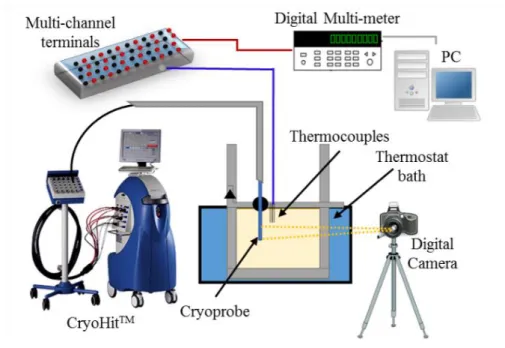
A schematic of the experimental apparatus is shown in Figs. 2.1, 2.2 and 2.3. A glass container (120 mm × 130 mm × 140 mm) comprising a tissue phantom was immersed in a bath controlled at 37C.

The tissue phantom (Fig. 2.3) comprised of a 0.9% sodium chloride aqueous solution, 3% gelatin (Wako), and 0.3% agarose-III (DojinDo). A J–T cryoprobe, cooled by supplying argon gas from a cylinder, was placed in the tissue phantom.

Figure 0.1 Experimental setup.

Figure 2.1 Experimental setup.

(26)

13

Figure 0.2 Container setup.

Figure 0.3 The setup inside the tissue phantom (a photo taken before starting the experiment).

A CryoHit^TM Needle I (Gallil Medical), a model that has been used worldwide, was used as the test probe. The probe comprised a 1.5-mm-diameter pipe with a sharp closed tip containing coiled capillary tubes. To monitor temperature variations at the cooled surface, T-

in diameter, were soldered onto the probe surface at distances 6 mm (tip side), 16 mm (middle), and 26 mm (base side) from the tip (Fig. 2.4). Another thermocouple was soldered onto the middle of the opposite surface.

The radial temperature distribution in the tissue phantom was also measured at the mid plane, approximately 16 mm from the tip, using 0.5-mm-diameter T-type sheath thermocouples. The

1．Cryoprobe 2．Thermocouple 3．Tissue phantom 4．Container 5．Thermostat bath 6．Lead wires 7．Gas supply

(27)

14

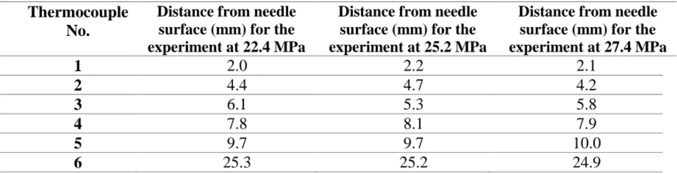
thermocouples emplaced through 18-Gauge guide needles at positions approximately 2, 4, 6, 8, 10, and 25 mm from the probe surface as shown in Fig. 2.5 and Table 2.1. The location of the thermocouple tip was precisely measured using a digital microscope (NIKKO NRM-D-2XZ). The voltage signals from the thermocouples were measured every 10 s using a digital multimeter (Agilent 34970A), recorded by computer, and converted to temperatures using a pre-calibrated conversion table (see Appendix A for calibration details). Photographs of the ice ball were taken using a digital camera. The size of the ice ball was then determined using a calibrated measure to correct the viewing angle. The refraction at the window was also compensated.

Figure 0.4 Cryoprobe with thermocouples attached on the surface.

Figure 0.5 Placement of thermocouples in tissue phantom.

Table 0.1 Distance from needle surface in the gelatin tissue phantom.

Thermocouple No.

Distance from needle surface (mm) for the experiment at 22.4 MPa

1 2.0 2.2 2.1

2 4.4 4.7 4.2

3 6.1 5.3 5.8

4 7.8 8.1 7.9

5 9.7 9.7 10.0

6 25.3 25.2 24.9

Figure 2.4 Cryoprobe with thermocouples attached on the surface.

Table 2.1 Distance from needle surface in the gelatin tissue phantom.

(28)

15

Experiments were conducted at 22.4, 25.2, and 27.4 MPa using the CryoHit system, which supplies argon gas through a connecting tube to the cryoprobe via a connecting port. The argon gas is then released to the atmosphere through the same port (CryoHit system is shown in Fig. 2.1). Each experiment was terminated 10 min after the start of cooling. The pressure drop monitored in the experiments was negligible in all cases. Three different cryoprobes (coded A, B, and C) were tested to check for any variation between products.

2.2 Numerical simulation

A two-dimensional numerical simulation was conducted for three purposes. The first was to validate the phase change model and the software by comparing the simulated results with those from experiments. Once it was validated, it could be used for estimating different conditions in the future.

The second was to calculate the cooling power that is difficult to be measured experimentally. The third was to examine the effect of blood perfusion. An apparent heat-capacity model, which is compatible with commercially available software, was used to model the phase change and consequent release of latent heat. The freezing phenomena was incorporated into a bioheat equation [54] but excluded metabolic heat. When applied to the two-dimensional radial coordinate system described in Fig. 2.6, the model was expressed as

 

1

b b b b

T T T

c kr k c T T Q

t r r r z z

          

   (2.1)

where T, t, ρ, c, and k are the temperature, time, density, specific heat capacity, and thermal conductivity, respectively. ωb is the rate of blood perfusion, and all values having the subscript b are those of blood.

The heat source Q was derived from the release of latent heat during freezing and is expressed as gs

Q L

 ^t

  ^(2.2)

where L is the latent heat and gs is the local solid fraction, defined by the ratio between the mass of ice and the total mass. Substituting Eq. (2.2) into Eq. (2.1), the following was obtained:

 

s 1

b b b b

g T T T

c L kr k c T T

T t r r r z z

     

        

           

 

   (2.3)

(29)

16

The blood-perfusion term was neglected in the simulation to compare with the experiments with the tissue phantom. It was incorporated into the simulation only for the purpose of examination of its effect on the results. The blood perfusion was assumed to be not exist (b = 0) in the partially and completely frozen regions. The freezing was assumed to be occurred in equilibrium with no diffusion and neglected the effect of the 3% gelatin and 0.3% agarose. The solid fraction was therefore determined from the phase-equilibrium diagram of the sodium chloride aqueous solution and given by

( ) ( )

eq s

eq

g T

T

 



  _(2.4)

where



is the mass fraction of sodium chloride in the bulk solution (



= 0.009) and _eq is the value on the liquidus line of the diagram at a given temperature. Based on the phase-equilibrium diagram, the freezing was assumed to be started at −0.5°C (gs = 0) and completed at −21.1°C (gs = 1). The thermophysical properties were estimated as a function of temperature taking the concentration into account.

The thermophysical properties of the partially frozen part (−21.1°C < T < −0.5°C) were treated with a mixture of pure ice and unfrozen liquid at the equilibrium mass fraction of sodium chloride. The thermophysical properties that are used in chapter 2 are displayed here as Eqs. 2.5-2.8 [79].

    

³ ²



7.0941 2089.4

7.0941 2089.4 1 0.0785 4.5417 105.09 4201.2

0.07168 0.07168

0.15993exp 4.16130 exp

2.61278 0.42045

0.4635 4149.4

s s

ap

T

g T g T T T

c T T

L T

 

      



        

 



{𝑇 < 𝑇_𝑙}

(2.5) {𝑇_𝑢 ≤ 𝑇 ≤ 𝑇_𝑙}

{𝑇 > 𝑇_𝑢}

    

²



0.0937 918.63

0.0937 918.63 1 0.1976 13.209 999.57 0.2249 1006.4

s s

T

g T g T T

T



 



       

  



{𝑇 < 𝑇_𝑙}

(2.6) {𝑇_𝑢≤ 𝑇 ≤ 𝑇_𝑙}

{𝑇 > 𝑇_𝑢}

(30)

17

  

964.9

1.0775 300.0

964.9

1.0775 1 0.0026 0.5648 300.0

0.0016 0.5641

s s

T

k g g T

T T

 

 

 

      

 





{𝑇 < 𝑇_𝑙}

(2.7) {𝑇_𝑢≤ 𝑇 ≤ 𝑇_𝑙}

{𝑇 > 𝑇_𝑢}

1.0

0.07168 0.07168

0.95013 0.41786 exp 1.74962 exp

2.61278 0.42045

0.0

s

T T

g

      

     



{𝑇 < 𝑇_𝑙}

(2.8) {𝑇_𝑢≤ 𝑇 ≤ 𝑇_𝑙}

{𝑇 > 𝑇_𝑢}

where cap, k, ρ, L and gs are specific heat capacity (J/(kg·K)), thermal conductivity (W/(m·K)), density (kg/m³), latent heat (J/kg), and solid fraction respectively. Tl (= −21.1°C) and Tu (= −0.53°C) are the lower and upper temperature limits of the partially frozen state.

Figure 2.6 shows the physical model and its coordinates with the origin set at the tip of the cryoprobe.

The initial temperature of the whole domain was set to 37°C. The probe surface was assumed to be at a uniform temperature (i.e. measured by experiment) across the cooled part 32 mm from the tip and adiabatic elsewhere. The temperature at the boundary of the solution domain was assumed to be 37°C.

The results were checked to confirm that the temperature gradient was zero at these boundaries. The average of the measured temperatures at the probe surface was used to derive the boundary condition as a function of time. Finite element method software was used to obtain the numerical solutions (MSC.Marc/Mentat).

Figure 2.6 Physical model for two-dimensional simulation.

(31)

18

Figure 0.6 Physical model for two-dimensional simulation.

2.3 Results and discussion

2.3.1 Observation of the ice ball

Figures 2.7(a)–(f) show photographs of the ice ball produced by probe B at 25.2 MPa, with a 5-mm- wide ruler used as a reference. Initially, the cylindrically frozen part was slightly larger near the tip with a neck appearing in the middle, reflecting the internal structure of the cryoprobe (Fig. 2.7(a)). This neck disappeared as the ice grew, and an ellipsoid shape was formed at 600 s (Fig. 2.7(f)). Similar growth processes were seen at different pressures. Although the overall shapes were similar, different probes produced ice balls with different lengths (Fig. 2.8). This apparently reflected structural differences between the positioning of capillaries inside the probes. However, this variation would be negligible in practice because the diameter of the ice ball was approximately the same in each case.

(a) 30 s (b) 60 s (c) 120 s

(d) 240 s (e) 420 s (f) 600 s

Figure 0.7 Growth of ice ball around probe B (25.2 MPa) (the width of ruler is 5 mm).

(a) 10 s (b) 300 s

Figure 0.8 Ice balls formed by different cryoprobes.

Figure 2.7 Growth of ice ball around probe B (25.2 MPa) (the width of ruler is 5 mm).

Figure 2.8 Ice balls formed by different cryoprobes.

(32)

19

Fig. 2.9 shows a comparison between the ice balls obtained by experiment and simulation at 25.2 MPa. The size and shape of the ice ball observed in the experiment agreed well with simulation that is shown in white dashed lines.

(a) 30 s (b) 60 s

(c) 120 s (d) 240 s

(e) 420 s (f) 600 s

Figure 0.9 Growth of ice ball around probe B (25.2 MPa). Dashed lines are the contour of ice ball obtained by simulation and the width of ruler is 5 mm.

2.3.2 Changes of temperature and frozen region

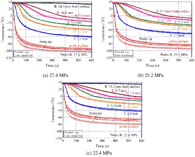
Figures 2.10(a)–(c) show the results at different pressures from the experiments using probe B. The measured temperatures at the designated positions are plotted by symbols. At all positions, the temperature fell as the gas pressure rose. At the probe surface, the lowest temperature was recorded at

Figure 2.9 Growth of ice ball around probe B (25.2 MPa). Dashed lines are the contour of ice ball obtained by simulation and the width of ruler is 5 mm.

(33)

20

the tip (shown by a cross). The red solid line near these symbols indicates the average of the surface temperatures measured at three positions from the tip. The average probe temperature dropped to −40°C within 40 s, even at 22.4 MPa, then more gradually declined towards the lowest temperature. While the temperature at the probe surface remained almost constant, it was decreasing at locations far from the probe. This suggests that the temperature distribution did not approach a steady state within 600 s. The lines in the figures at the designated positions indicate the simulation results. At all positions, the results agreed well with the experimental data.

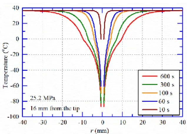
Fig. 2.11 shows the radial temperature distribution obtained by simulation at different time points (i.e. 10, 60, 100, 300, and 600 s) around the cryoprobe at 25.2 MPa. The temperature distributions were obtained at 16 mm from the tip. The temperature distribution at 600 s shows that the temperature is lower at the middle of the cooling part of the cryoprobe and the temperature gradient change was very small at the probe surface. This reflects the results of the temperature change in Fig. 2.10 (b).

(a) 27.4 MPa (b) 25.2 MPa

(c) 22.4 MPa

Figure 0.10 Experimentally measured temperature change of probe B at different locations in the tissue phantom and different gas pressures. The symbols show the experimental data, and the lines show the simulation results.

Figure 2.10 Experimentally measured temperature change of probe B at different locations in the tissue phantom and different gas pressures. The symbols show the experimental data, and the lines show the simulation results.

(34)

21

Figure 0.11 The radial temperature distribution obtained by simulation at different time points.

Figure 2.12 compares three replications of the probe B experiments. The temperature measured at the probe surface, ~2 mm from the surface, and ~10 mm from the surface agreed well with each other, demonstrating that the experimental results were replicable.

Figure 2.13 compares the average temperatures of the three different probes. The surface temperatures of probes B and C agreed well with each other, whereas that of A was higher by ~5 K.

The difference is not simply due to the lower gas pressure of probe A, but may reflect the fact that the cooling region was displaced by a few millimeters from that of the other probes (Fig. 2.8(a)) while the temperature measurement points were fixed. The variation between probes was insignificant, particularly on terms of the diameter of the ice ball that will be discussed later in Fig. 16(a).

Figure 0.12 Comparison of replicated experiments using probe B.

Figure 2.11 The radial temperature distribution obtained by simulation at different time points.

Figure 2.12 Comparison of replicated experiments using probe B.

(35)

22

Figure 0.13 Comparison of average surface temperatures of different probes.

Figure 2.14 shows the temperature distribution along the probe. The temperature at the tip was lower than that at the middle and base, particularly in the early stage of cooling. In Fig. 2.14 there was a difference in the longitudinal temperature distribution at probe surface between probe B and C. This reflected the different structure of the probes, and the difference reduced to approximately 10 K at 600 s.

Figure 2.15 shows the average probe temperature as a function of the gas pressure. The probe temperature linearly decreased as the gas pressure increased and was not time dependent. The lowest temperature achieved by probe B was ~−95C at 27.4 MPa, ~−5C at 25.2 MPa and ~−5C at 22.4 MPa.

Figure 0.14 Longitudinal temperature distribution at probe surface.

Figure 2.13 Comparison of average surface temperatures of different probes.

Figure 2.14 Longitudinal temperature distribution at probe surface.

(36)

23

Figure 0.15 Average probe temperature as a function of gas pressure.

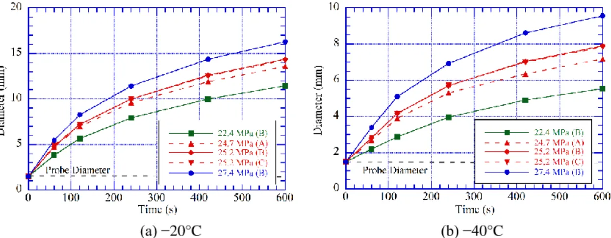
Figures 2.16 (a) and (b) show the size of the ice ball as a function of time. As the temperature did not reach a steady state (Fig. 2.10), it was unsurprising that the ice ball was still growing when the experiment terminated. After 600 s, the diameter of the ice ball reached 27 mm at 27.2 MPa, 25 mm at 25.2 MPa, and 21 mm at 22.4 MPa. No significant difference was found in the diameter of the ice ball formed by probes A, B, and C, but the ice balls formed by probes A and C had a length ~3 mm longer than that of probe B. At pressures greater than 25 MPa, the length of the ice ball around every probe exceeded 45 mm.

(a) Diameter (b) Length

Figure 0.16 Size of ice ball as a function of time.

From the thermal engineering point of view, the goal in cryosurgery is not to produce an ice ball larger than the target tissue but to expose the complete tissue to a lethal temperature. Figures 2.17 (a) and (b) show the development of isotherms at −C and −C over time in the radial direction. The

Figure 2.15 Average probe temperature as a function of gas pressure.

Figure 2.16 Size of ice ball as a function of time.

(37)

24

effect of pressure was qualitatively similar to that on the diameter of the ice front shown in Fig. 2.16(a), but the values were considerably smaller. Even at 27.4 MPa, they were only 16 mm at −C (Fig. 2.17 (a)) and 9 mm at −C (Fig. 2.17 (b)). Therefore, a tissue whose lethal temperature is −C would be damaged by freezing only in a limited region near the probe. This suggests that two or more probes should be simultaneously used to treat tumors larger than 10 mm as will be discussed later in Chapter 3. Fig. 2.18 shows the development of isotherms in the axial direction.

(a) −20°C (b) −40°C

Figure 0.17 Position of the lethal temperatures as a function of time (radial direction).

(a) −20°C (b) −40°C

Figure 0.18 Position of the lethal temperatures as a function of time (axial direction).

Figure 2.17 Position of the lethal temperatures as a function of time (radial direction).

Figure 2.18 Position of the lethal temperatures as a function of time (axial direction).

(38)

25

2.3.3 Temperature distribution in the frozen region

Figures 2.19 (a) and (b) show the measured temperature in the frozen region as a function of radial position at 400 s and 600 s, respectively. After 350 s from the start of cooling, the temperature distribution of a straight line on this semi-logarithmic graph was formed except in the vicinity of the probe and can be well approximated by

1

ln

2

T = C r +C

(2.9)

As the analytical solution for the steady state has the same form, this suggests that the non-steady effect becomes negligibly small at the periphery of the ice.

Figure 2.20 shows the radial temperature distribution in the ice ball, which was obtained from Eq.

(2.9) with specific coefficients C1 and C2 for each condition. To highlight the temperature at the periphery of the ice ball and to determine the appropriate safety margin, the distance from the ice front is shown as a function of the temperature. This figure demonstrates that the distance from the ice surface at a given temperature increased with time, because the temperature gradient near the surface declined as the ice ball grew. The key result is that at higher sub-zero temperatures, the surface temperature distribution was similar under different pressures.

(a) 400 s (b) 600 s

Figure 0. 19 Radial temperature distribution.

Figure 2.19 Radial temperature distribution.

(39)

26

Figure 0.20 Distance from ice front as a function of temperature.

The coefficients C1 and C2 in Eq. (2.9) were determined at each 50 s interval, and the ice front−C) and the locations at C and C, which are usually taken to be the lethal temperatures for typical cancer cells, were determined. Figure 2.21(a) shows the distance between the ice front and these locations as a function of time. This represents the safety margin required to guarantee that the temperature of the target tissue will be lower than the lethal temperature. The safety margin almost increased linearly with time and was not significantly different at different pressures. At 600 s from the start of cooling, the isotherm at −C was located ~5 mm inside the ice front while that at −C was ~8 mm inside. Figure 2.21(b) shows the size of safety margin as a function of the ice ball radius. This figure may be used to estimate the safety margin during cryosurgical procedures for an ice ball of a specific size, as measured from the MRI images.

(a) Margin size as a function of time (b) Margin size as a function of the radius of ice ball

Figure 0.21 Location at assumed lethal temperatures in terms of the distance from the ice surface.

Figure 2.20 Distance from ice front as a function of temperature.

Figure 2.21 Location at assumed lethal temperatures in terms of the distance from the ice surface.

(40)

27

Figure 2.22 shows the radial position at given temperatures relative to the ice surface, i.e., r40/rice

and r20/rice, as a function of the ice ball radius. The values of r40/rice and r20/rice became larger at higher pressures because of the difference in temperature at the probe surface. However, the value did not significantly depend on the radius of the ice ball, as r20/r_ice0.6 and r40/r_ice0.35 at 27.4 MPa.

When a freezing time longer than 10 min is used, Fig. 2.22 is more useful than Fig. 2.21(b) because the safety margin should be estimated by extrapolating each curve.

Figure 0.22 Radial position at assumed lethal temperatures relative to the radius of the ice ball.

2.3.4 Effect of blood perfusion

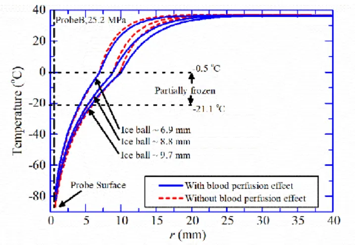
This research set out to provide guidelines for determining a safety margin based on experiments using a tissue phantom. However, the effect of blood perfusion could also be significant during cryosurgery and was therefore examined by simulation. Figure 2.23 compares the temperature distributions with and without blood perfusion, assuming the same temperature change at the probe surface shown in Fig. 2.10(b). The thermal effect of blood perfusion was assumed to be

40 kW / (m3 K)

b bc b 

  , which was large enough for soft tissues [70]. The growth of ice ball was slower when blood perfusion was included. However, if we compare the temperature distribution between with and without blood perfusion, the temperature inside the ice ball was similar at ice ball sizes of approximately 6.9, 8.8, and 9.7 mm, while it was different in the unfrozen part. This is because that the blood perfusion does not occur in the frozen part and this result has been predicted in an earlier paper [79], which simulated tissue with an assumed doubling of the original thermal conductivity. The results confirmed that the values shown in Fig. 2.21(b) and Fig. 2.22 can be used to estimate the safety

Figure 2.22 Radial position at assumed lethal temperatures relative to the radius of the ice ball.

(41)

28

margin for a given size of ice ball irrespective of the presence and magnitude of blood perfusion. In the present chapter, the multiplier for the thermal conductivity in the heat conduction equation was determined by comparing the temperature distribution inside the ice ball with that calculated from the bioheat equation. This was based on the hypothesis that the bioheat equation provides actual temperature distribution inside living tissues. However, there is only a few studies, including the first paper by Pennes [54], which measured temperature distribution in vivo. Therefore, we expect to have non-invasive methods for measuring temperature distribution in living tissues, which definitely contributes to medical treatments.

Figure 0.23 Comparison of the radial temperature distribution with and without blood perfusion.

2.3.5 Cooling power

Although cryoprobes are widely used as cooling devices, their cooling power has not been provided, because this is difficult to be determined experimentally. Therefore, we investigated the cooling power using simulations of probe B by integrating the local heat flux at the probe surface over the whole area.

The cooling power rapidly increased after the start of cooling and approached a constant value (Fig.

2.24). This value, which can be considered as the rated power, was approximately 16 W at 22.4 MPa, 21 W at 25.2 MPa, and 24 W at 27.4 MPa.

Figure 2.23 Comparison of the radial temperature distribution with and without blood perfusion.

(42)

29

Figure 0.24 Cooling Power as a function of time. Figure 2.24 Cooling Power as a function of time.

(43)

30

Chapter 3 Freezing with two parallel cryoprobes

The research work in Chapter 3 particularly focuses on providing an experimental validation of the cooling performance of the cryoprobe in the case of using two parallel cryoprobes at the same time, which is not studied before in the previous literature.

Results in this chapter presents ice ball sizes, safety margins, comparisons with the single probe experiments, and guidelines for the usage of the Joule-Thomson cryoprobe for successful two-probe cryosurgery applications. Experimental data in chapter 3 were obtained from a previous research work in the laboratory [80].

3.1 Experimental apparatus and methods

The experimental apparatus and method were basically the same as those used in Chapter 2. The tissue phantom was prepared in a container and then immersed in a water bath (Figs. 3.1 and 3.2). Two cryoprobes used in Chapter 2 were placed in the tissue phantom at a given center-to-center distance (~10 mm or ~20 mm) using a holder at the top of the container. At the cooling surface, 50-m-diameter T-type thermocouples were also soldered at three different locations (6 mm, 16 mm, and 26 mm from the tip) to monitor the temperature change for both of the cryoprobes (Fig. 2.4).

(44)

31

(a) ~10 mm center-to-center distance (b) ~20 mm center-to-center distance

The temperature distribution in the tissue phantom was also measured using 0.5-mm-diameter K- type sheath thermocouples (Fig. 3.3). Three thermocouples (coded 0, 1, and 2) were placed in the middle plane between two probes, one at the center and the others at ~3 mm and ~6 mm from the center.

Another three thermocouples (coded 3, 4, and 5) were placed at ~1.5 mm, ~10 mm, and ~24 mm from the cryoprobe to measure outward temperature distribution. The actual locations of the thermocouples were precisely measured using the digital reading-microscope described in chapter 2. The center-to- center distance between two cryoprobes that was measured using the microscope was 10.7 mm and 20.4 mm. The experiment was conducted at the argon gas pressure of 25.2 MPa. Each experiment was terminated 10 min after the start of cooling.