LaPlace
方程式一般境界値問題の直接近似解法
茨城大学理学部 大西和榮 (Kazuei Onishi)
Department of
Mathematical
Sciences,Ibaraki University
九州情報大学経営情報学部 大浦洋子 (Yoko Ohura)
Kyushu Institute of Information
Sciences
We propose in this paper a unified treatment of conventional boundary value problem, the Cauchy
problem, and under- or over-determined problems of the Laplace equationin two-dimensional
domain enclosed by the smooth curve. The Dirichlet data can be prescribed on any part of
the boundary, while the Neumann data can be prescribed on any other part ofthe boundary.
This problemis reformulated in terms of the variationalproblem with aleast-square functional,
which is thenrecastinto primary and adjoint boundary value problems of the Laplace equation.
A non-iterative numerical method of solution usingthe BEMis presented. Numerical examples
suggest that our treatment is effective.
Key Words: Inverseproblem, Boundaryvalue identification, Direct method
1. Introduction
Let $\Omega$ be a simply connected bounded domain with
its smooth boundary $\Gamma$ in $R^{2}$. Let
$n$ be the exterior
normal to the boundary.
We consider the Laplace equation;
$-\triangle u(X)=0$, $x\in\Omega$ (1)
subject to Dirichlet andNeumanndata;
$u|\mathrm{r}_{u}=\overline{u}$ and $\frac{\partial u}{\partial n}=q|_{\Gamma_{q}}=\overline{q}$ (2)
given on respective non-zero measurepartsof the
bound-ary$\Gamma_{u}$and$\Gamma_{q}$. Herewe notice that thecomponents $\Gamma_{u}$
and $\Gamma_{q}$ can be taken arbitrarily to some extent. This
problem setting encompasses the conventional mixed
boundary value problem, the Cauchy problem,
under-andover-determinedproblemsof theLaplaceequation.
Fromthisreason we call theproblem the general or
in-verseboundary valueproblem.
If the solution of the problem eqns (1), (2) exists,
the solution $u$ at internal points of the domain can be
expressed by Green’s formula;
$u( \xi)=\int_{\Gamma}G(X;\xi)q(x)d\Gamma(X)$
$- \int_{\Gamma}\frac{\partial G}{\partial n}(x;\epsilon)u(x)d\Gamma(X)$, $\xi\in\Omega$ (3)
where$G(x;\xi)$is the fundamental solutiontothe
Lapla-cian;
$-\triangle G(x;\epsilon)=\delta(X-\xi)$ (4)
with the Dirac measure6at the point$\xi$. In two
dimen-sions we know
$G(x; \xi)=\frac{1}{2\pi}\ln\frac{1}{||x-\xi||}$ . (5)
The boundary values $u|\mathrm{r}$ and$q|\mathrm{r}$ should satisfy the
boundaryintegral equation;
$\frac{1}{2}u(\xi)+\int_{\Gamma}\frac{\partial G}{\partial \mathrm{n}}(x;\epsilon)u(X)d\Gamma(X)$
$= \int_{\Gamma}G(x;\epsilon)q(x)d\Gamma(X)$, $\xi\in\Gamma$. (6) In preceding $\mathrm{P}^{\mathrm{a}}\mathrm{P}^{\mathrm{e}\mathrm{r}\mathrm{s}}(1),(2)$ the authors presented
an
iterativemethod for numerical solution of the problem
eqns (1), (2). However, our problem is essentially
lin-ear. The authors feel that linear problems should be
solved in principle without iteration. In thispaper an
attempt ispresentedat anapproximatesolution ofthe
problem using the boundary element method without
theiteration.
2.
Variational
ProblemLet $\Gamma_{u}^{c}$ and $\Gamma_{q}^{c}$ be complement sets of $\Gamma_{u}$ and $\Gamma_{q}$,
respectively. We recast the problem eqns (1), (2) into
the following variationalproblem: Find$u|\Gamma_{u}^{\mathrm{c}}=\omega$ that
minimizes the functional
$J( \omega)=\int_{\Gamma_{q}}|q(x;\omega)-\overline{q}(x)|^{2}d\mathrm{r}(X)$
$+ \eta\int_{\Gamma}|q(x;\omega)|2d\Gamma(X)$ (7)
subject to
$-\triangle u(x;\omega)=0$, $x\in\Omega$ (8)
$u|\mathrm{r}_{u}=\overline{u}$ and $u|\Gamma_{u}^{\mathrm{c}}=\omega$. (9)
The second term on the right hand side ofeqn (7)is the
Tikhonov regularizer with the regularizationparameter
$\eta>0$ in order to make the problem well-posed. Here
We discuss some mathematical questions about the
existence and the uniqueness of the solution $\omega$ of the
variational problem in whichthefunctional $J(\omega)$attains
its minimum. The first theorem states that our
under-determinedproblem is quasi-controlable (3).
..
Theorem 1 The convex set
$\{q(\omega)=\frac{\partial u}{\partial n}|_{\Gamma_{u}^{\mathrm{C}}}/$ $\triangle u=0$ in $\Omega$, $u\in H^{1/2}(\Gamma)$
$\mathrm{s}.\mathrm{t}$. $u|\Gamma_{\mathrm{u}}=0$, $u|\Gamma_{u}^{\mathrm{C}}=\omega\in H^{1/2}(\Gamma^{\mathrm{c}}u)\}$
is dense in $H^{-1/2}(\Gamma_{u}^{c})$.
Proof Weconsider a bounded linear operator $I\mathrm{t}’$by
definition:
$K$: $H^{1/2}( \mathrm{r}_{u}^{c})\ni\omegarightarrow\frac{\partial u}{\partial\tau},(x;\omega)\in H^{-1/2}(\mathrm{r}_{u}^{\mathrm{c}})$
.
In orderto provethattherange of$I\zeta$is densein$H^{-1/2}(\Gamma_{u}^{c})$, it sufficesustoshowthat the adjoint operator$I\mathrm{c}^{\prime \mathrm{r}}$is an injection ($\mathrm{o}\mathrm{n}\mathrm{e}- \mathrm{t}_{0}$-onemap).
We wiu find $I\mathrm{e}’’$ from the definition:
$\langle IC\omega, \varphi\rangle=\langle\omega, K^{*}\varphi\rangle$ for $\forall\varphi\in H_{0}^{1/2}(\Gamma^{c})u$
.
For given $\varphi\in H_{0}^{1/2}(\Gamma_{\mathrm{u}}^{\mathrm{C}})$, we consider the boundary
valueproblem:
$\Delta\psi(x)=0$, $x\in\Omega$
subject to $\psi|_{\Gamma_{u}}=0$, $\psi|_{\Gamma_{u}^{\mathrm{c}}}=\varphi$.
$\tau$
The solution $\emptyset(x)$ exists uniquely in $H^{3/2}(\Omega)$. From
Green’sintegral theorem, we have
$0= \int_{\Omega}(\triangle u)\psi_{d}\Omega$
$= \int_{\Gamma}\frac{\partial u}{\partial n}\psi_{d}\Gamma-\int_{\Gamma}u\frac{\partial\psi}{\partial n}d\Gamma+\int_{\Omega}u\triangle\psi d\Omega$
$= \int_{\Gamma_{u}^{\mathrm{C}}}\frac{\partial u}{\partial n}\varphi d^{-}\mathrm{r}-\cdot i^{\omega\frac{\partial\psi}{\partial n}}\Gamma cud\Gamma$
.
$-$
This implies that
$\int_{\Gamma_{\mathrm{u}}^{\mathrm{c}}}\frac{\partial u}{\partial n}\varphi d\Gamma=\int_{\Gamma_{u}^{\mathrm{c}}}\omega\frac{\partial\psi}{\partial n}d\Gamma$ for
$\forall\varphi\in H_{0}^{1/2}(\Gamma^{c})u$.
.
Weknow nowthat
$I\mathrm{e}^{-l}$ : $H^{1/2}0( \mathrm{r}^{c}u)\ni\varphirightarrow\frac{\partial\psi}{\partial n}\in L^{2}(\Gamma_{u}^{c})$
We will show that $K^{*}$is injective. Let$IC^{\mathrm{r}} \varphi=\frac{\partial\psi}{\partial n}=$
$0$. Tothis end,weconsider the boundary value problem:
$\triangle\psi(x)=0$, $x\in\Omega$
subject to $\emptyset|\mathrm{r}_{\mathrm{u}}=0$, $\frac{\partial\psi}{\partial n}|\Gamma_{u}^{\mathrm{c}}=0$
.
This problem is uniquely solvable with the solution$\psi(x)$
$=0$ in $\Omega$. Therefore we obtain $\varphi=\psi=0$on$\Gamma_{u}^{c}$.
$\square$
This theorem guarantees that our variational problem is solvable for almost all $u|\mathrm{r}$ and$q|\mathrm{r}$.
Theorem 2 The Fre’chetderivative$J’(\omega)$in$L^{2}(\Gamma_{u}^{c})-$
senseis givenby
$J’( \omega)|\mathrm{r}_{u}\mathrm{c}=\frac{\partial v}{\partial \mathrm{z}},(x)$
.
(10)Proof We see $J(\omega+\delta\omega)-J(\omega)$ $= \int_{\Gamma_{q}}\{|q(x;\omega+\delta\omega)-\overline{q}(x)|^{2}-|q(x;\omega)-\overline{q}(x)|^{2}\}d\Gamma$ $+ \eta\int_{\Gamma}\{|q(X;\omega+\delta\omega)|^{2}-|q(x_{\mathrm{i}}\omega)|^{2}\}d\Gamma$ $= \int_{\Gamma_{q}}\{q(X;\omega+\delta\omega)+q(x;\omega)-2\overline{q}(X)\}$ $\{q(x;\omega+\delta\omega)-q(X;\omega)\}d\Gamma$ $+ \eta\int_{\Gamma}\{q(X;\omega+\delta\omega)+q(x;\omega)\}$ $\{q(x;\omega+\delta\omega)-q(X;\omega)\}d\Gamma$ $= \int_{\Gamma_{\mathrm{q}}}\{q(X;\omega+\delta\omega)-q(X;\omega)$ +2 $[q(x;\omega)-\overline{q}(x)]\}\delta q(x;\omega)d\Gamma$ $+ \eta\int_{\Gamma}\{q(x;\omega+\delta\omega)-q(x;\omega)$ +2$q(x;\omega)\}\delta q(x;\omega)d\Gamma$
$= \int_{\Gamma_{q}}2[q(x;\omega)-\overline{q}(X)]\delta q(x;\omega)d\Gamma+\int_{\Gamma_{q}}|\delta q(X;\omega)|^{2}d\Gamma$
$+ \eta\int_{\Gamma}2q(x;\omega)\delta q(X_{1}^{\cdot}\omega)d\Gamma+\eta\int_{\Gamma}|\delta q(x;\omega)|2d\Gamma$
$= \int_{\Gamma_{q}}2[(1+\eta)q(x;\omega)-\overline{q}(X)]\delta q(x;\omega)d\mathrm{r}$
$+ \int_{\Gamma_{q}^{\mathrm{c}}}2\eta q(x;\omega)\delta q(x;\omega)d\Gamma$
$+ \int_{\Gamma_{q}}(1+\eta)|\delta q(x;\omega)|^{2}d\Gamma+\int_{\Gamma_{q}^{\mathrm{c}}}\eta|\delta q(X|.\omega)|^{2}d\Gamma$.
In theabove,weput$\delta u(x;\omega)=u(x;\omega+\delta\omega)-u(x;\omega)$,
andaccordingly$\delta q(x;\omega)=q(x;\omega+\delta\omega)-q(x;\omega)$. We
notice that $\triangle(\delta u)=0$in$\Omega,$ $\delta u=0$on$\Gamma_{u},$ and$\delta u=\delta\omega$ on$\Gamma_{u}^{c}$.
We now consider $v\in H^{2}(\Omega)$ as a solution of the
Laplaceequati on
$-\triangle v(x;\omega)=0$, $x\in\Omega$ (11)
subject to the boundary conditions
$v|_{\Gamma_{q}}=2\{(1+\eta)q(x;\omega)-\overline{q}(X)\}$
and $v|_{\Gamma_{q}^{\mathrm{c}}}=2\eta q(x;\omega)$
.
(12)From Green’s integraltheorem;
$\int_{\Omega}(\triangle v)\delta ud\Omega=\int_{\Gamma}\frac{\partial v}{\partial n}\delta ud\Gamma-\int_{\Gamma}v\frac{\partial\delta u}{\partial n}d\Gamma+\int_{\Omega}v\triangle(\delta u)d\Omega$,
we have
$0= \int_{\Gamma_{\mathrm{u}}^{\mathrm{c}}}\frac{\partial v}{\partial n}\delta\omega d\Gamma-\int_{\Gamma_{q}}2[(1+\eta)q(x;\omega)-\overline{q}(x)]\delta qd\Gamma$
Consequently we obtain
$J(\omega+\delta\omega)-J(\omega)$
$= \int_{\Gamma_{u}^{\mathrm{c}}}\frac{\partial v}{\partial n}\delta\omega d\Gamma$
$+ \int_{\Gamma_{\mathrm{q}}}(1+\eta)|\delta q(X;\omega)|^{2}d\Gamma+\int_{\Gamma_{q}^{\mathrm{c}}}\eta|\delta q(X^{\cdot}\omega)||^{2}d\Gamma$
$=( \frac{\partial v}{\partial n},$
$\delta\omega)_{L}2\mathrm{t}^{\Gamma_{u})}c)+o(||\delta\omega||$
.
Corollary The second-order derivative$J”(\omega)$is given
by
$J^{\prime/}( \omega)\delta\omega|\Gamma^{\mathrm{c}}u=2\frac{\partial w}{\partial \mathrm{n}}(x;\delta q)$ (13)
with $w\in H^{2}(\Omega)$ as a solution of the Laplace equation $-\triangle w(x;\delta q)=0$, $x\in\Omega$ (14)
subject to the boundary conditions;
$w|\mathrm{r}_{q}=(1+\eta)\delta q$ and $w|_{\Gamma_{q}^{c}}=\eta\delta q$
.
(15)Proof We start with theexpression
$J(\omega+\delta\omega)=J(\omega)+(J’(\omega), \delta\omega)_{L^{2}}(\Gamma_{u}C)$
$+ \int_{\Gamma_{q}}(1+\eta)|\delta q(X;\omega)|^{2}d\mathrm{r}$
$+ \int_{\Gamma_{q}^{\mathrm{c}}}\eta|\delta q(X;\omega)|2d\Gamma$
.
(16)From Green’s integral theorem;
$\int_{\Omega}(\triangle w)\delta ud\Omega=\int_{\Gamma}\frac{\partial w}{\partial \mathrm{n}}\delta ud\Gamma$
$- \int_{\Gamma}w\frac{\partial\delta u}{\partial \mathrm{n}}d\Gamma+\int_{\Omega}w\triangle(\delta u)d\Omega$,
we have
$0= \int_{\Gamma_{u}^{\mathrm{c}}}\frac{\partial w}{\partial n}\delta wd\Gamma$
$- \int_{\Gamma_{q}}(1+\eta)\cdot|\delta q|2d\Gamma-\int_{\Gamma_{q}^{c}}\eta|\delta q|2d\Gamma$
.
Consequentlywe obtain
$J(\omega+\mathit{5}\omega)=J(\omega)+(J’(\omega), \delta\omega)_{L^{2}(}\Gamma^{\mathrm{c}})u$
$+ \frac{1}{2}\int_{\Gamma_{u}^{\mathrm{c}}}2\frac{\partial w}{\partial n}\delta\omega d\Gamma$
$=J(\omega)+(J’(\omega), \delta\omega)_{L^{2}}(\mathrm{r}_{u}\mathrm{C})$
$+ \frac{1}{2}(J’’(\omega)\delta\omega, \delta\omega)L^{2}(\Gamma^{\mathrm{c}})u$.
Thenext theoremstates the unique existence of the
minimizer of the functional $J(\omega)(4)$.
Theorenl 3 Tlle functional $J$ : $H^{1/2}(\Gamma_{u}^{\mathrm{C}})\ni\omega$ $rightarrow$
$R_{+}$ isstrictly convex.
Proof For $\omega_{k}(k=1,2)$,let$u(x;\omega_{k})$ be the solution
ofthe boundary value problem:
$\triangle u=0$ $\mathrm{i}\mathrm{I}1$ $\Omega$, $u|\mathrm{r}_{\mathrm{u}}=\overline{u}$, $u|\Gamma_{u}^{\mathrm{C}}=\omega_{k}$.
Foranynumber$\theta(0<\theta<1)$,we note that$\theta u(x;\omega_{1})+$
$(1-\theta)u(x;\omega_{2})$isalso thesolution of the boundaryvalue
problemwith$u|\Gamma_{\mathrm{u}}^{c}=\theta\omega_{1}+(1-\theta)\omega_{2}$due to the linearity
of the problem. Using the convexity of the parabola
$\{\theta\tau_{1}+(1-\theta)\tau_{2}\}2<\theta\tau_{1}^{2}+(1-\theta)\tau_{2}2$forany $\tau_{1},$$\tau_{2}\in R$,
we see
$J(\theta\omega_{1}+(1-\theta)\omega 2)$
$= \int_{\Gamma_{q}}|\theta q(X;\omega_{1})+(1-\theta)q(X;\omega 2)-\overline{q}(X)|2d\Gamma$
$+ \eta\int_{\Omega}|\nabla\{\theta u(X;\omega 1)+(1-\theta)u(x;\omega 2)\}|^{2}d\Omega$
$= \int_{\Gamma_{q}}|\theta\{q(x;\omega 1)-\overline{q}(X)\}$
$+(1-\theta)\{q(X;\omega_{2})-\overline{q}(x)\}|2d\mathrm{r}$
$+ \eta\int_{\Omega}|\theta\nabla u(x;\omega_{1})+(1-\theta)\nabla u(x;\omega_{2})|2d\Omega$
$\leq\int_{\Gamma_{\mathrm{q}}}\{\theta|q(x\cdot\omega_{1})-\overline{q}(X)||^{2}$
$+(1-\theta)|q(x;\omega 2)-\overline{q}(x)|2\}d\Gamma$
$+ \eta\int_{\Omega}\{\theta|\nabla u(x;\omega 1)|2+(1-\theta)|\nabla u(X;\omega_{2})|2\}d\Omega$
$=\theta J(\omega_{1})+(1-\theta)J(\omega_{2})$.
Thisimplies that $J(\omega)$ is convex. To showthat $J(\omega)$is
strictly convex, we can see that
$\frac{1}{2}(J^{\prime/}(\omega)\delta\omega, \delta\omega)_{L(}2\Gamma_{\mathrm{u}}\mathrm{c})$
$=$ $\int_{\Gamma_{u}^{\mathrm{c}}}\frac{\partial w}{\partial n}\delta\omega d\Gamma$
$=$ $\int_{\Gamma_{q}}(1+\eta)|\mathit{5}q|^{2}d\Gamma+\int_{\Gamma_{q}^{C}}\eta|\delta q|2d\Gamma>0$ :
if and only if$\delta\omega\neq 0$in $H^{1/2}(\Gamma_{u}^{c})$
.
$-$.$\square$
3. Boundary Elenlent Metllod
We divide the whole boundary $\Gamma$into the series of$n$
boundaryelements as $\Gamma\simeq\Gamma^{h}=\bigcup_{j=1j}^{n}\Gamma$ forits
approx-imation, where $h$ stands for some representative size
ofthe boundary elements. Here the boundary element
subdivision should bein accordance with theboundary
components $\Gamma_{u}$ and $\Gamma_{q}$.
We approximate the boundary values $u|_{\Gamma}$ and $q|_{\Gamma}$
byintroducing theinterpolation functions$N_{j}(x)$ inthe
form;
$u| \mathrm{r}\simeq u^{h}(x)=\sum_{j=\iota}^{n}Nj(X)u_{j;}$, (17)
$q|_{\Gamma} \simeq q^{h}(x)=.\sum_{J=1}^{n}N_{j()q_{j}}X$, $x\in\Gamma$ (18)
with approximate nodal values $u_{j}$ and$q_{\mathrm{J}}$
. to the exact
nodal values$u(x_{j})$and$q(x_{j})$,respectively, atthenodes
$x_{\mathrm{J}}$ $(j=1,2, \cdots , n)$ on the boundary F. We
form; In the similar way we write
$v| \mathrm{r}\simeq v^{h}(x)=\sum_{j=1}^{n}N_{j(}X)v_{j}$ , (19)
$r| \mathrm{r}\simeq r^{h}(x)=\sum_{j=1}^{n}N_{j}(x)rj$, $\dot{x}\in\Gamma$ (20)
with approximate nodal values $v_{j}$ and $r_{j}$ to the exact
$v(x_{j})$ and$r(x_{j})$, respectively,at$x_{j}$ onF.
The exactboundaryvalues$u|\mathrm{r}$and$q|\mathrm{r}$ in the
bound-ary integral equation (6) are replaced by the
approxi-mations $u^{h}|\mathrm{r}$ and $q^{h}|\mathrm{r}$ of eqns (17), (18) respectively.
Thisyields
$\frac{1}{2}u(\xi)+\sum_{j=1}^{n}\int_{\Gamma}\frac{\partial G}{\partial n}(X;\xi)Nj(x)d\mathrm{r}(X)u_{j}$.
$= \sum_{j=1}^{n}\int_{\mathrm{r}}c(x;\xi)N_{j(X})d\Gamma(X)qj$, $\xi\in\Gamma.(21)$
We take those$n$nodes$x_{j}$ again as collocation points
in order to fully discretize the boundary integral
equa-tion (21). Put$\xi=x\dot{.}$ $(i=1,2, \cdots , n)$. Then wehave
$\frac{1}{2}u_{i}+\sum_{j=1}^{n}\int\Gamma)\frac{\partial G}{\partial n}(X;xi)N_{j}(X)d\Gamma(Xu_{j}$
:
$= \sum_{j=1}^{n}\int_{\Gamma}G(x;X.)N_{j}(x)d\Gamma(x)qj$, (22)
$\{v\}=$
$n_{2}\mathrm{n}_{2}^{\mathrm{c}}$ ,$\{r\}=$
$ll_{1}^{c}n_{1}$.
(28)Then thesystems eqns (23) and (26) canbe written
respectivelyin the partitionedform;
$n_{1}$ $n_{1}^{c}$ $n[H_{1}^{(1)}H_{2}^{(1)}]$ $n_{2}^{\mathrm{c}}$ $n_{2}$ $=[G_{1}^{(1)}$ $G_{2}^{(1)}]$ (29) and $,\iota_{2}$ $\mathrm{n}_{2}^{\mathrm{c}}$ $n[H_{1}(2)H_{2}(2)]$ $n_{1}$ $n_{1}^{\mathrm{c}}$ $=[G_{1}^{(2)}G_{2}^{(2)}]$ , (30)
where numbers of rows and columns of the coefficient matrices are indicated.
which results in the system of linear equations in the
matrixform; 4.
Direct
Method ofSolution$[H]\{u\}=[G]\{q\}$ (23)
$\mathrm{w}\mathrm{i}$th eachenti ty
$h_{ij}= \frac{1}{2}\delta_{1j}+\int_{\Gamma}\frac{\partial G}{\partial n}(x;x|)Nj(X)d\Gamma(X)$, (24)
$g. \cdot j=\int_{\Gamma}G(x;x.\cdot)N\mathrm{j}(X)d\Gamma(X)$ , (25)
for$i,$$j=1,2,$$\cdots$ ,$n$. Here,$\delta_{ij}$ is theKroneckersymbol.
Weapplythediscretizingprocedureagaintothe
bound-aryintegral equation corresponding to theadjoint
prob-lem eqns (11), (12) to obtain
$[H]\{v\}=[G]\{r\}$ (26)
withthesame$n\cross n$ coefficientmatrices $[H]$and$[G]$ as
in eqn(23).
We denoteby $n_{1}$ the number of nodeson$\Gamma_{\mathrm{u}}$, and by
$n_{2}$ thenumber of nodes on $\Gamma_{q}$, respectively. Let $n_{1}^{c}=$ $n-n_{1}$ and $n_{2}^{c}=n-n_{2}$, being the respective numbers
of nodes on $\Gamma_{u}^{\mathrm{c}}$ and $\Gamma_{q}^{c}$. According to the respective boundary components $\Gamma_{\mathrm{u}}$ and$\Gamma_{q}$ we write the column
vectors$\{u\}$ and $\{q\}$in the$\dot{\mathrm{f}}\mathrm{o}\mathrm{r}\mathrm{m};$ ’
We insertboundaryconditions of primary andadjoint
problemsinto the partitioned systems of eqns (29), (30):
From eqn (9) we have
$\{u_{1}\}=\{\overline{u}_{1}\}$, $\{u_{2}\}=\{\omega\}$
.
(31)From eqn (12) wehave
$\{v_{1}\}=2\eta\{q1\}$, $\{v_{2}\}=2((1+\eta)\{q2\}-\{\overline{q}_{2}\})$,
(32)
and from eqn (10) as the necessary condition that $J(\omega)$
is minimal wehave
$\{r_{2}\}=\{0\}$. (33)
Therefore the systems eqns (29), (30) reduce to the
form; $[H_{1}^{(1)}$ $H_{2}^{\langle 1)}]$ $=[G_{1}^{(1)}$ $G_{2}^{(1)}]$ (34) and $\{u\}=n_{1}n_{1}^{c}$ , $-$ $\iota$ $\{q\}=n_{2}n_{2}^{c}$ , (27)
where $n_{1}$ nodal values $u_{j}$ on $\Gamma_{u}$ arecollected in $\{u_{1}\}$, andthe$n_{1}^{\mathrm{c}}$nodal values on$\Gamma_{u}^{c}$in$\{u_{2}\}$, whereas$n_{2}$nodal
values$qj$ on$\Gamma_{q}$ are collected in $\{q_{2}\}$, and the $n_{2}^{c}$ nodal
valueson$\Gamma_{q}^{c}$in $\{q_{1}\}arrow$
$[H_{1}^{(2)}$
$H_{2}^{\{2)}]$
$=[G_{1}^{(2)}$ $G_{2}^{(2)}]$ , (35)
We combine eqns (34) and (35). We take unknown
nodal values to theleftof the equation to obtain
$n_{2}^{c}$ $n_{1}^{c}$ $n_{1}$ $n_{2}$ $nn$ $-G_{1}^{(2)}$ 2 $(1+\eta)H^{\mathrm{t}}22)]$ $n_{1}$ $n_{2}$ $=$ $nn$
(a)
48
boundary nodesWe notice that the coefficient matrix on the left hand
side of the augmented newsystemof lineareqns(36) is
squareof order $2n$.
5. Nunlerical Exanlples
Suppose tllat the harmonic function
$u(x_{1}, x_{2})=x_{1}^{2}-x_{2}^{2}=’\cdot\cos(22\theta)$ (37)
with the polar coordinates $x_{1}=r\cos\theta,$ $x_{2}=f\sin\theta$
serves as a solution of theinverse boundary value
prob-lem eqns (1), (2) in the unitcircle;
(b)
96
boundary nodesFig. 2
Boundary elements$\Omega=\{(\uparrow\cdot, \theta)|0\leq r<1,0\leq\theta<2\pi\}$ (38)
as shownin Fig. 1
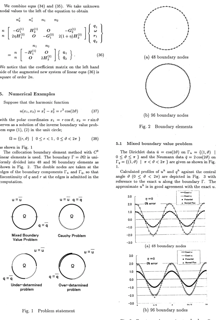
The collocation boundary element method with $C^{0}$
linear elements is used. The boundary $\Gamma=\partial\Omega$ is
uni-formly divided into 48 and 96 boundary elements as
shown in Fig. 2. The double nodes are taken at the
edges of the boundary components$\Gamma_{u}$ and $\Gamma_{q}$, so tliat
discontinuity of$q$and$r$ at theedges is admitted inthe
computation.
5.1 Mixed boundary value problem
The Dirichlet data $\overline{u}=\cos(2\theta)$ on $\Gamma_{u}=\{(1, \theta)$ $|$
$0\leq\theta\leq\pi\}$ and the Neumanndata $\overline{q}=2\cos(2\theta)$ on $\Gamma_{q}=\{(1, \theta)|\pi<\theta<2\pi\}$ aregiven as shown in Fig.
1.
Calculated profiles of $u^{h}$ and $q^{h}$ against $\mathrm{t}1_{1}\mathrm{e}$
central
angle $\theta(0\leq\theta<2\pi)$ are depicted in Fig. 3 with
reference to the exact $u$ along the boundary F. The
approximate $u^{h}$ is ingood agreement with the exact
$u$
.
$\mathrm{u}=\overline{\mathrm{u}}$ $\mathrm{u}=\overline{\mathrm{u}}\mathrm{q}=\mathrm{q}-$ 3.0 2.0 1.0 0.0 $-1.0$MixedBoundary CauchyProblem
ValueProblem
$-2.0$
$-3.0$
$\mathrm{U}\mathrm{n}\mathrm{d}\mathrm{e}\ulcorner \mathrm{d}\mathrm{e}\mathrm{t}\mathrm{e}\mathrm{r}\mathrm{m}\mathrm{i}\mathrm{n}\mathrm{e}\mathrm{d}$ $\mathrm{O}_{\mathrm{V}\mathrm{e}\ulcorner}\mathrm{d}\mathrm{e}\mathrm{t}\mathrm{e}\mathrm{r}\mathrm{m}\mathrm{i}\mathrm{n}\mathrm{e}\mathrm{d}$
problem problem
Fig.
1
Probleln statement (b)96
boundarynodes5.2 Cauclly probleln
The Cauchy data $\overline{u}=\cos(2\theta)$ and $\overline{q}=2\cos(2\theta)$ on
$\Gamma_{u}=\Gamma_{q}=\{(1, \theta) |0\leq\theta\leq\pi\}$aregiven as shown in
Fig. 1.
Calculated profiles of $n^{h}$ and $q^{h}$ against the central
angle $\theta(0\leq\theta<2\pi)$ are depictedin Fig. 4 with
refer-ence to theexact $u$ and $q$along the boundary $\Gamma$. Both
of the approximate $u^{h}$ and $q^{h}$ are in good agreement
respectivelv with the exact $u$and$q$.
3.0 2.0 1.0 0.0 $-1.0$ $-2.0$ $-3.0$
Fig.
4
Exact $u,$ $q$ alld approximate $u^{h},$ $q^{h}$ on$\Gamma$ (a) $\eta=0$ 3.0 2.0 1.0 0.0 $-1.0$ $-2.0$ $-3.0$ (b) $?_{l}=0.37$
Fig.
5
$\mathrm{L}^{\urcorner}(\mathrm{x}_{\dot{\mathfrak{c}}}\mathrm{t}\mathrm{c}\mathrm{t}u,$$//$and approximate
$u^{h},$ $q^{h}$on
$\Gamma$$\underline{\circ|\mathrm{b}\mathrm{h}}$
$\underline{\Phi}$
$\fallingdotseq^{\mathrm{r}_{\prec}}$
Fig.
6
Hansen’s L-curve5.3 Under-determined problem
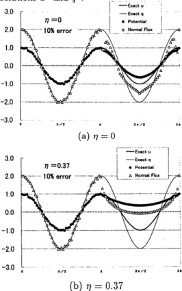
The Dirichlet data $\overline{u}=\cos(2\theta)$ on $\Gamma_{u}=\{(1, \theta)|$ $0\leq\theta\leq\pi/2\}$ and the Neumann data$\overline{q}=2\cos(2\theta)$ on $\Gamma_{q}=\{(1, \theta)|\pi<\theta<3\pi/2\}$ are given as shown in
Fig. 1.
Calculated proffies of$u^{h}$ and $q^{h}$ against the central
angle $\theta(0\leq\theta<2\pi)$ aredepicted in Fig. 7 with
refer-ence to the exact $u$ and $q$ along the boundary $\Gamma$. The
approximate $u^{h}$ isin fairly good agreement on
$\Gamma_{q}$, and
the approximate$q^{h}$is infairly good agreement on$\Gamma_{\mathrm{u}}$.
3.0 2.0 1.0 0.0 $-1.0$ $-2.0$ $-3.0$
(a) 48 bouuldarynodes
3.0 2.0 1.0 0.0 $-1.0$ $-2.0$ $-3.0$ (b)
96
boundary nodes5.4 Over-determilled problem References
The Dirichlet data $\overline{u}=\cos(2\theta)$ on $\Gamma_{u}=\{(1, \theta)|$
$0\leq\theta\leq\pi\}$ and the Neumanm data $\overline{q}=2\cos(2\theta)$ on $\Gamma_{q}=\{(1, \theta)|\pi/2<\theta<3\pi/2\}$are given as shownin
Fig. 1.
Calculated profiles of $u^{h}$ and $q^{h}$ against the central
angle $\theta(0\leq\theta<2\pi)$ are depicted in Fig. 8 with
refer-ence to the exact $u$ and $q$ along the boundary F. The
approximate $u^{h}$ is in good agreement on $\Gamma_{q}\backslash \Gamma_{u}$, and theapproximate$q^{h}$ isin good agreement on$\Gamma_{u}\backslash \Gamma_{q}$.
3.0
2.0
1.0 0.0
$-1.0$
(1) Onishi, K., Kobayashi, K.,andOhura, Y.,
Numer-ical solution of aboundaryinverse problem ofthe
Laplaceequation. Theoretical and Applied
Mechan-ics, NCTAM, Vol.45, pp.257-264 (1996).
(2) Ohura, Y., Kobayashi, K.,andOnishi, K.,
Numeri-calsolutionofan under-determinedproblem of the
Laplace equation. Journal
of
Applied Mechtanics,JSCE, Vol.2, pp.185-189 (1999).
(3) Lions, J. L., Contr\^ole Optimal $d,e$ Syst\‘emes
Gou-vern\’es par des
\’Equations
aux D\’eriv\’ees Partielles,Dunod, Paris (1968).
(4) Ekeland, I., andTemam, R., Convex Analysis and
Variational Problems, North-Holland Publishing
Company, Amsterdam (1976).
(5) Hansen, P. C., Analysis of discrete ill-posed
prob-lems by means of the L–curve. SIAM Reviews,
Vol.34, No.4, $\mathrm{p}\mathrm{p}.561-580$ (1992).
$-2.0$
$-3.0$
(a)
48
boundarynodes3.0 2.0 1.0 0.0 $-1.0$ $-2.0$ $-3.0$ (b)
96
boundary nodesFig.
8
Exact $u,$ $q$ and approximate $u^{h},$ $q^{h}$ on $\Gamma$6.
Conclusions
A boundary inverse problem is considered for the
Laplace equation in two dimensions. By introducing
a convex functionaltobeminimized, the solution of the
inverseproblem is understood as the minimizer of the
functional. The necessary condition for the functional
to attain the minimum is paraphrased by the primary
and adjoint boundary value problems of the Laplace
equation. The boundary element method is applied to
obtain numerical solution of the problems, yielding an
augumented system of linear algebraic equations. The
linearsystem of equations can be solved directly. Four
test examples suggest the validity of this directmethod