Bifurcation
Structure
of Positive
Stationary
Solutions for
a
Lotka-Volterra
Competition
Model
with
Diffusion I:
Numerical
Verification
of
Local Structure
Yukio Kan-on
Department
of
Mathematics,
Faculty
of Education
Ehime University, Matsuyama, 790-8577,
Japan
kanonQed.
ehime-u.
$\mathrm{a}\mathrm{c}$.
jp
1. Introduction
This
paper
is
concerned
with the
bifurcation structure of positive
solu-tions for
the
stationary problem
(1.1)
$\{$
$0=\epsilon D\mathrm{u}’’+\mathrm{f}(\mathrm{u})$
,
$x\in(\mathrm{O}, \pi)$
,
$\mathrm{u}^{l}=0$
,
$x=0,\pi$
of
a
Lotka-Volterra
competition-diffusion system,
where
$D=\mathrm{d}\mathrm{i}\mathrm{a}\mathrm{g}(d_{u}, d_{v})$,
$\mathrm{u}=(u, v)$
,
$\mathrm{f}(\mathrm{u})=(f,g)(\mathrm{u})$
,
$f(\mathrm{u})=f^{0}(\mathrm{u})u$
,
$g(\mathrm{u})=g^{0}(\mathrm{u})v$
,
every parameter is positive, and
we
call
$\mathrm{u}(x)=(u, v)(x)$
positive when
$u(x)$
and
$v(x)$
are
positive for any
$x\in[0, \pi]$
.
From the competitive
interaction,
we
may
assume
that
$\mathrm{f}^{0}(\mathrm{u})=(f^{0},g^{0})(\mathrm{u})$
is
a
smooth function in
$\mathrm{u}$and satisfies
$f_{v}^{0}(\mathrm{u})<0$
,
$g_{u}^{0}(\mathrm{u})<0$
for
any
$\mathrm{u}\in \mathbb{R}_{+}^{2}$,
where
$\mathbb{R}_{+}=(0, +\infty)$
.
As
$\mathrm{f}^{0}(\mathrm{u})$is
represented
as
$f^{0}(\mathrm{u})=f_{0,0}^{0}+f_{n_{1},0}^{0}u^{n_{1}}+f_{0,n_{2}}^{0}v^{\mathrm{n}_{2}}+\mathrm{t}\mathrm{h}\mathrm{e}$
remainder
term,
$g^{0}(\mathrm{u})=g_{0,0}^{0}+g_{n_{S},0}^{0}u^{ns}+g_{0,n_{4}}^{0}v^{n_{4fl}}+\mathrm{t}\mathrm{h}\mathrm{e}$
remainder
term
with suitable
constants
$f_{i,j}^{0},$ $g_{i,j}^{0}$and
$n_{j}$
,
we
treat the simplest nonhnearity
$f^{0}(\mathrm{u})=1-u^{n}-cv^{n}$
,
$g^{0}(\mathrm{u})=1-bu^{n}-v^{n}$
to discuss the bifurcation structure of positive solutions for
(1.1),
where
$n$
,
$b$
and
$c$
are
positive
constants. At
this point,
it is
obvious
that
(1.1)
has
constant solutions
$(0,0),$ $(0,1),$ $(1,0)$
,
and
\^u
$(=( \hat{u},\hat{v}))=((\frac{1-c}{1-bc})^{\underline{\mathit{1}}}’$
.
$,$
$( \frac{1-b}{1-bc})^{\frac{1}{n}})$
which is positive
for
either
$\max(b, c)<1$
or
$\min(b,c)>1$
.
First of all,
let
us
consider
the
case
$\min(b, c)<1$
.
Suppose that
(1.1)
has
a
positive solution
$(u,v)(x)$
.
Setting
$u(x_{-}^{u})= \min u(x)$
,
$x\in[0,\pi]$
$v(x^{\underline{\nu}})= \min v(x)$
,
$x\in[0,\pi]$
we
have
$u(x_{+}^{u})= \max_{x\in[0,\pi]}u(x)$
,
$v(x_{+}^{v})= \max_{x\in[0,\pi]}v(x)$
,
$1-u(x_{-}^{u})^{n}-cv(x_{+}^{v})^{n}\leq 0\leq 1-bu(x_{-}^{u})^{n}-v(x_{+}^{v})^{n}$
,
$1-bu(x_{+}^{u})^{n}-v(x_{-}^{v})^{n}\leq 0\leq 1-u(x_{+}^{u})^{n}-cv(x_{-}^{v})^{n}$
by
virtue
of the
functional
form of
$\mathrm{f}^{0}(\mathrm{u})$.
By
the above inequalities,
we
obtain
$0<(1-c)v(x_{+}^{v})^{n}\leq(1-b)u(x_{-}^{u})^{n}\leq 0$
for
the
case
$c<1\leq b$
,
$0<(1-b)u(x_{+}^{u})^{n}\leq(1-c)v(x_{-}^{v})^{n}\leq 0$
for the
case
$b<1\leq c$
.
This contradiction implies
that
(1.1)
has
no
positive
solutions
for
either
$c<1\leq b$
or
$b<1\leq c$
.
fiom
$u(x_{+}^{u})^{n}-u(x_{-}^{u})^{n}\leq c(v(x_{+}^{v})^{n}-v(x_{-}^{v})^{n})\leq bc(u(x_{+}^{u})^{n}-u(x_{-}^{u})^{n})$
,
we find
out that
$u(x)$
and
$v(x)$
must be
constant
in
$x$
for
the
case
$\max(b, c)<$
$1$
.
Hence
we see
that
(1.1)
has
no
positive
nonconstant solutions for the
case
$\min(b,c)<1$
.
Next, let
us
consider the
case
$\mu=(b,c)\in \mathcal{M}\equiv\{(b,c)|\min(b,c)>1\}$
.
It
is
easy
to check that
$\mathrm{u}=\hat{\mathrm{u}}$is an
unstable equihbrium
point
of the
ODE
$\mathrm{u}_{t}=\mathrm{f}(\mathrm{u})$,
and
that
for
each
$n\in \mathbb{R}_{+}$
and
$\mathrm{d}=(d_{u},d_{v})\in D(n,\mu)$
,
the
lin-earized operator of
(1.1)
around
$\mathrm{u}=\hat{\mathrm{u}}$has the only eigenvalue
(respectively,
at
least
two
eigenvalues)
with positive
real part for any
$\epsilon>1$
(respectively,
$0<\epsilon<1)$
,
where
$D(n,\mu)=\{\mathrm{d}\in \mathrm{R}_{+}^{2}|\det(-D+\mathrm{f}_{\mathrm{u}}(\hat{\mathrm{u}}))=0\}$
.
In brief,
$D(n,\mu)$
consists
of
$\mathrm{d}\in \mathbb{R}_{\vdash}^{2}$such that the linearized
operator with
$\epsilon=1$
has the eigenvalue
$0$
whose eigenfunction
is of the form
$\pm \mathrm{v}\cos x$
,
where
$\mathrm{v}$is
a
nontrivial solution of
$(-D+\mathrm{f}_{\mathrm{u}}(\text{\^{u}}))$
$\mathrm{v}=0$
.
The
bifurcation
theory
gives
us
the fact that positive nonconstant solutions of
(1.1)
which
look
$\mathrm{l}\mathrm{i}\mathrm{k}\mathrm{e}\pm \mathrm{v}\cos(kx)$perturbations from
$\mathrm{u}=\hat{\mathrm{u}}$bifurcate at
$\epsilon=1/k^{2}$
for any
fixed
$n\in \mathbb{R}_{+},$
$\mathrm{d}\in D(n, \mu)$
and
$k\in \mathbb{N}$
.
As
the
multiple
existence
of positive
nonconstant
solutions
for
(1.1)
is suggested,
one
important problem
is
to
seek all
positive
solutions
of (1.1). In this
paper,
as a
first
step
to
answer
the problem,
we
shall establish the local bifurcation structure of positive
solutions of
(1.1)
with
respect
to
$\epsilon$for suitably fixed
$\rho=$
(
$n$
,
la,
d).
We
define
the
$\mathrm{r}\mathrm{e}\mathrm{l}\mathrm{a}\mathrm{t}\mathrm{i}\mathrm{o}\mathrm{n}\prec \mathrm{b}\mathrm{y}$$(u_{1},v_{1})\prec(u_{2}, v_{2})\Leftrightarrow u_{1}<u_{2},$
$v_{1}>v_{2}$
,
and
set
Al
$= \bigcup_{+(n,\mu)\in \mathrm{R}\mathrm{x}\Lambda 4}\{(n,\mu)\}\mathrm{x}D(n, \mu)$
,
$N_{2}=\{\rho\in N|n\geq 2\}$
,
$E_{0}(\rho)=\mathbb{R}_{+}\mathrm{x}$
{\^u},
$X=\{\mathrm{u}(.)\in C^{2}([0,\pi])|\mathrm{u}’(\mathrm{O})=0=\mathrm{u}’(\pi)\}$
.
For each
$\rho\epsilon N$
, we
denote
by
$E(\rho)$
the
set
of
$(\epsilon, \mathrm{u}(.))\in \mathbb{R}_{+}\mathrm{x}X$
such that
$\mathrm{u}(x)$
is
a
positive
solution of
(1.1)
for
$\epsilon$,
and
by
$E_{k}(\rho)(k\in \mathrm{N})$
the
set of
$(\epsilon, \mathrm{u}(.))\in E(\rho)$
such that
there
exists
$\ell\in\{0,1\}$
such that
$(-1)^{j+\ell}\mathrm{u}’(x\rangle\succ 0$
holds on
$(\pi j/k, \pi(j+1)/k)$
for
any
integer
$0\leq j<k$
.
By
definition,
we
have
$\bigcup_{k\geq 0}E_{k}(\rho)\subset E(\rho)$
for any
$\rho\in N$
, and
see
that
$(\epsilon, \mathrm{u}(.))\in E_{k}(\rho)$
is
equivalent
to
$(k^{2}\epsilon, \mathrm{u}(./k))\in E_{1}(\rho)$
for any
$\rho\in N$
and
$k\in$
N.
LEMMA
1.1
([1]).
$E( \rho)=\bigcup_{k\geq 0}E_{k}(\rho)$
holds
for
any
$\rho\in N$
.
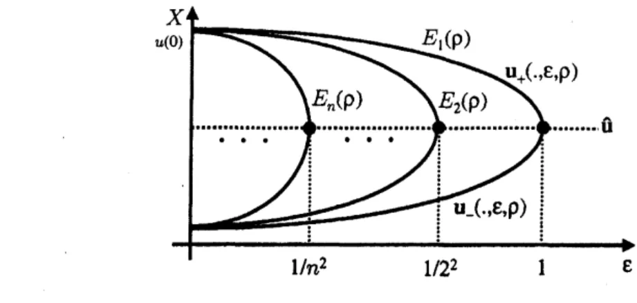
FIGURE 1. Global Bifurcation Structure.
The above lemma
says
that
for
each
$\rho\in N$
, we can
understand
the
complete
structure
of
$E(\rho)$
by using the
information on
the structure of
$E_{1}(\rho)$
.
In consideration of
results
in [1] and [2],
we
may
have
the
following
conjecture:
CONJECTURE
1.2. For any
$\rho\in N$
, there enist continuous
functions
$\mathrm{u}-(., \epsilon,\rho)$
and
$\mathrm{u}_{+}(.,\epsilon,\rho)$
such
that
(i)
$E_{1}(\rho)=\{(\epsilon, \mathrm{u}_{\pm}(., \epsilon, \rho))|\epsilon\in(0,1)\}$
,
(ii)
$\pm \mathrm{u}_{\pm}’(x,\epsilon,\rho)\prec 0$
for
any
$(x,\epsilon)\in(0, \pi)\cross(0,1)$
,
and
(iii)
$\lim_{\epsilonarrow 1}\mathrm{u}_{\pm}(., \epsilon,\rho)=\hat{\mathrm{u}}$
.
Figure
1
shows
the
bifurcation
structure of
positive
solutions
for (1.1)
which
is suggested by the above conjecture. In this paper, to get at the truth
of
the above conjecture,
we
shall
establish
the following
result
by
employing
the numerical
verification:
THEOREM
1.3.
For each
$\rho\in N_{2}$
, theoe exist
a constant
$\nu_{0}(\rho)>0$
and
$C^{2}$
-class jfunctions
$\epsilon_{0}(\nu,\rho),$
$\mathrm{u}0(., \nu,\rho)$
defined
on
the interval
$(-\nu_{0}(\rho), \nu_{0}(\rho))$
such that
(i)
$(\epsilon \mathrm{o}(\nu,\rho),$$\mathrm{u}_{0}(., \nu,\rho))\in E_{1}(\rho)$
holds
for
each
$\nu_{j}$and
(ii)
$\epsilon_{0}(0,\rho)=1,$
$\tau_{\nu}^{\epsilon \mathrm{o}(0,\rho)}\theta=0and_{\overline{\partial}\overline{\nu}^{\mathrm{F}}}\partial^{2}\epsilon \mathrm{o}(0,\rho)<0$are
satisfied.
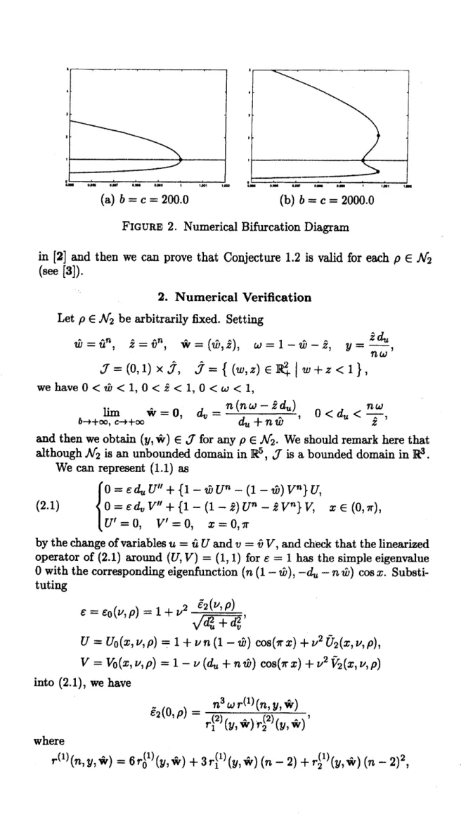
Figure 2
shows
numerical
bifurcation
diagrams
for
the
case
where
$n=1.1$
and
$d_{u}=d_{v}$
are
satisfied.
The
horizontal and vertical
axes mean
the
value
of
$\epsilon$and
$u(\mathrm{O})/\hat{u}$
,
respectively.
Fhrom this figure,
we find
out that there
exists
a
subregion
of
$N$
such
that
Conjecture
1.2
is not valid.
In this paper, to
determine the geometrical
position
on
the
curve
of
positive
nonconstant
solutions
for
(1.1)
bifurcating from
$\mathrm{u}=$
\^u
at
$\epsilon=1$
,
we
employ the
numerical verification
method such
as
the
interval arithmetic
built into Mathematica. Unfortunately,
when
we
change
$\mathrm{f}^{0}(\mathrm{u})$for
$f^{0}(\mathrm{u})=1-u^{n_{1}}-\mathrm{c}v^{n_{2}}$
,
$g^{0}(\mathrm{u})=1-bu^{n_{8}}-v^{n_{4}}$
with positive
constants
$b,$
$c$
and
$n_{j}$
, we
have not
succeeded
in establishing
the
geometrical
position,
so
that the
bifurcation
structure
for
(1.1)
with
more
general nonlinearity
is
stil
open.
In the next section,
we
shall discuss
the
numerical
method to verify the
(a)
$b=c=l$
UU.U
(b)
$\mathit{0}=c=\mathrm{Z}\mathrm{U}\mathrm{U}\mathrm{U}.\mathrm{U}$FIGURE 2. Numerical
Bifurcation Diagram
in
[2]
and then
we
can
prove that Conjecture
1.2
is
valid for
each
$\rho\in N_{2}$
(see
[3]).
2.
Numerical Verification
Let
$\rho\in N_{2}$
be arbitrarily
fixed.
Setting
$\hat{w}=\hat{u}^{n}$
,
$\hat{z}=\hat{v}^{n}$
,
IRr
$=(\hat{w},\hat{z})$
,
$\omega=1-\hat{w}-\hat{z}$
,
$y= \frac{\hat{z}d_{u}}{n\omega}$,
$J=(0,1)\cross\hat{J}$
,
$\hat{J}=\{(w, z)\in \mathbb{R}_{+}^{2}|w+z<1\}$
,
we
have
$0<\hat{w}<1,0<\hat{z}<1,0<\omega<1$
,
$\lim_{barrow+\infty,carrow+\infty}\hat{\mathrm{w}}=0$
,
$d_{v}= \frac{n(n\omega-\hat{z}d_{u})}{d_{u}+n\hat{w}}$
,
$0<d_{u}< \frac{n\omega}{\hat{z}}$
,
and then
we
obtain
$(y,\hat{\mathrm{w}})\in J$
for any
$\rho\in N_{2}$
.
We
should remark here
that
although
$N_{2}$
is
an
unbounded domain in
$\mathbb{R}^{5},$$J$
is
a bounded domain
in
$\mathbb{F}$.
We
can
represent
(1.1)
as
(2.1)
$\{$
$0=\epsilon d_{u}U’’+\{1-\hat{w}U^{n}-(1-\hat{w})V^{n}\}U$
,
$0=\epsilon d_{v}V’’+\{1-(1-\hat{z})U^{n}-\hat{z}V^{n}\}V$
,
$x\in(0,\pi)$
,
$U’=0$
,
$V^{j}=0$
,
$x=0,\pi$
by the
change of variables
$u=\hat{u}U$
and
$v=\hat{v}V$
,
and check
that
the
linearized
operator
of
(2.1)
around
$(U, V)=(1,1)$
for
$\epsilon=1$
has the simple eigenvalue
$0$
with
the corresponding eigenfunction
$(n(1-\hat{w}), -d_{u}-n\hat{w})\cos x$
.
Substi-tuting
$\epsilon=\epsilon_{0}(\nu,\rho)=1+\nu^{2}\frac{\tilde{\epsilon}_{2}(\nu,\rho)}{\sqrt{d_{\mathrm{u}}^{2}+d_{v}^{2}}}$
,
$U=U_{0}(x, \nu,\rho)=1+\nu n(1-\hat{w})\cos(\pi x)+\nu^{2}\tilde{U}_{2}(x, \nu,\rho)$
,
$V=V_{0}(x, \nu,\rho)=1-\nu(d_{u}+n\hat{w})\cos(\pi x)+\nu^{2}\tilde{V}_{2}(x, \nu,\rho)$
into
(2.1),
we
have
$\tilde{\epsilon}_{2}(0,\rho)=\frac{n^{3}\omega \mathrm{r}^{(1)}(n,y,\hat{\mathrm{w}})}{\mathrm{r}_{1}^{(2)}(y,\hat{\mathrm{w}})\mathrm{r}_{2}^{(2)}(y,\hat{\mathrm{w}})}$
,
where
and
the
functions
$r_{j}^{(1)}$and
$r_{j}^{(2)}$are
shown
in Appendix.
After
simple
cal-culations,
we
obtain
$\mathrm{r}_{1}^{(2)}(y,\hat{\mathrm{w}})>0$
and
$r_{2}^{(2)}(y,\hat{\mathrm{w}})>0$
for any
$(y,\hat{\mathrm{w}})\in J$
.
Hence
it follows that
the denominator of
$\tilde{\epsilon}_{2}(0,\rho)$is positive for
any
$\rho\in N_{2}$
.
Hereafter,
we
shall
discuss
the numerical
method to verify
$r_{k}^{(1)}(y,\hat{\mathrm{w}})<0$
for
any
$(y,\hat{\mathrm{w}})\in J$
and
$k\in K\equiv\{0,1,2\}$
.
Without loss of
generality,
we
may
assume
ab
$\leq\hat{z}$by
changing the
role
between
$u$
and
$v$
if
necessary. From
$r_{0}^{(1)}(0,\hat{\mathrm{w}})=-3\hat{w}^{4}\hat{z}^{4}$
,
$r_{0}^{(1)}(1,\hat{\mathrm{w}})=-3(1-\hat{w})^{4}\hat{z}^{2}(1-\hat{z})^{2}$
,
$\mathrm{r}_{1}^{(1)}(0,\hat{\mathrm{w}})=-3\hat{w}^{4}\hat{z}^{4}$
,
$\mathrm{r}_{1}^{(1)}$(
$1$
,
if)
$=-3(1-\hat{w})^{4}\hat{z}^{2}(1-\hat{z})^{2}$
,
$\mathrm{r}_{2}^{(1)}(0,\hat{\mathrm{w}})=-\hat{w}^{4}\hat{z}^{4}$
,
$\mathrm{r}_{2}^{(1)}(1,\hat{\mathrm{w}})=-(1-\hat{w})^{4}\hat{z}^{2}(1-\hat{z})^{2}$
,
we
obtain
$r_{k}^{(1)}(y,\hat{\mathrm{w}})<0$
for
any
$y$
in
a
neighborhood of
$y=0$
and
$y=1$
for
each
$\hat{\mathrm{w}}\in J$
and
$k\in K$
.
Let
$k\in K$
be
arbitrarily
fixed.
First of
all, let
us
consider the
case
where
$\hat{\mathrm{w}}$is close
to the
origin. By
$r_{0}^{(1)}(y,\hat{\mathrm{w}})=-4y^{4}(y-1)(y-2)+o(1)$
,
$r_{1}^{(1)}(y,\hat{\mathrm{w}})=-y^{4}(y-1)(4y-10)+o(1)$
,
$r_{2}^{(1)}(y,\hat{\mathrm{w}})=-y^{4}(y-1)(4y-7)+o(1)$
as
$\hat{\mathrm{w}}arrow \mathrm{O}$,
we
should
remark here that
$\mathrm{r}_{k}^{(1)}(y,\hat{\mathrm{w}})$is
degenerate
at
$(y,\hat{\mathrm{w}})=$
$(0,0)$
.
Since
$r_{k}^{(1)}(y, \hat{\mathrm{w}})=\sum_{j=0}^{6}r_{k,j}^{(1)}(\hat{\mathrm{w}})y^{j}$
satisfies
$r_{k,0}^{(1)}(\hat{\mathrm{w}})=\tilde{r}_{k,0}^{(1)}\hat{w}^{4}\hat{z}^{4}(1+o(1))$
,
$\tilde{\mathrm{r}}_{0,0}^{(1)}=-3$,
$\tilde{r}_{1,0}^{(1)}=-3$
,
$\tilde{r}_{2,0}^{(1)}=-1$
,
$\mathrm{r}_{k,1}^{(1)}(\hat{\mathrm{w}})=\tilde{r}_{k,1}^{(1)}\hat{w}\hat{z}^{3}(1+o(1))$
,
$\tilde{r}_{0,1}^{(1)}=-4$
,
$\tilde{r}_{1,1}^{(1)}=-6$
,
$\tilde{\gamma}_{2,1}^{(1)}=-3$
as
$\hat{\mathrm{w}}arrow \mathrm{O}$,
it follows
that
$p_{k}^{(1)}(y, \hat{\mathrm{w}})\equiv-\frac{r_{k,0}^{(1)}(\hat{\mathrm{w}})+r_{k,1}^{(1)}(\hat{\mathrm{w}})y}{y^{2}}$
is positive
and strictly decreasing in
$y\in \mathrm{R}_{+}$
for
each
$\hat{\mathrm{w}}\in\hat{J}_{k,1}^{-}$, where
$\hat{J}_{k,1}^{-}=\{\hat{\mathrm{w}}\in\hat{J}|\max(r_{k,0}^{(1)}(\hat{\mathrm{w}}),$
$r_{k,1}^{(1)}(\hat{\mathrm{w}}))<0\}$
.
Setting
$p_{k}^{(2)}(y, \hat{\mathrm{w}})=\sum^{4}\ell=0\mathrm{r}^{(1)}k,\ell+2(\hat{\mathrm{w}})y^{\ell}$
,
we
have
$p_{k}^{(2)}(1,\hat{\mathrm{w}})<p_{k}^{(1)}(1,\hat{\mathrm{w}})$
for
any
$\hat{\mathrm{w}}\in\hat{J}$because of
$r_{k}^{(1)}(y,\hat{\mathrm{w}})=y^{2}(p_{k}^{(2)}(y,\hat{\mathrm{w}})-p_{k}^{(1)}$
(
$y$
,
Siii
)
$)$
.
As iii
$arrow 0$
, we
obtain
$\tau_{\nu}^{p_{k}(1,\hat{\mathrm{w}})=2\tilde{\Gamma}_{k_{)}4}+3\tilde{r}_{k,5}^{(1)}+4\tilde{r}_{k,6}^{(1)}+o(1)}\theta(2)(1)>0$
,
$\frac{p_{k}^{(2)}(\hat{z},\hat{\mathrm{w}})}{\hat{z}^{2}}=\tilde{\mathrm{r}}_{k,2}^{(1)}+\tilde{\mathrm{r}}_{k,3}^{(1)}+\tilde{\mathrm{r}}_{k,4}^{(1)}+o(1)<0$
,
because of
$r_{k,2}^{(1)}(\hat{\mathrm{w}})=\tilde{r}_{k,2}^{(1)}\hat{z}^{2}(1+o(1))$
,
$\tilde{r}_{0,2}^{(1)}=-8$
,
$\tilde{r}_{1,2}^{(1)}=-10$
,
$\tilde{r}_{2,2}^{(1)}=-7$
,
$r_{k,3}^{(1\rangle}(\hat{\mathrm{w}})=\tilde{r}_{k,3}^{(1)}\hat{z}(1+o(1))$
,
$\tilde{r}_{0,3}^{(1)}=14$
,
$\tilde{r}_{1,3}^{(1)}=10$
,
$\tilde{r}_{2,3}^{(1)}=-4$
,
$\mathrm{r}_{k,4}^{(1)}(\hat{\mathrm{w}})=\tilde{r}_{k,4}^{(1)}+o(1)$
,
$\tilde{r}_{0,4}^{(1)}=-8$
,
$\tilde{r}_{1,4}^{(1)}=-10$
,
$\tilde{r}_{2,4}^{(1)}=-7$
,
$\tau_{k,5}^{(1)}(\hat{\mathrm{w}})=\tilde{r}_{k,5}^{(1)}+o(1)$
,
$\tilde{r}_{0,5}^{(1)}=12$
,
$\tilde{r}_{1,5}^{(1)}=14$
,
$\tilde{r}_{2,5}^{(1)}=11$
,
$r_{k,6}^{(1)}(\hat{\mathrm{w}})=\tilde{\mathrm{r}}_{k,6}^{(1)}+o(1)$
,
$\tilde{\mathrm{r}}_{0,6}^{(1)}=-4$,
$\tilde{r}_{1,6}^{(1)}=-4$
,
$\tilde{r}_{2,6}^{(1)}=-4$
.
Since
$p_{k}^{(1)}(y,\hat{\mathrm{w}})$
is positive
and
decreasing
in
$y\in \mathbb{R}_{\vdash}$
for each
$\hat{\mathrm{w}}\in\hat{J}_{k,1}^{-}$,
we
have
$p_{k}^{(2)}(y,\hat{\mathrm{w}})<p_{k}^{(1\rangle}(y,\hat{\mathrm{w}})$
for
any
$\hat{\mathrm{w}}\in\hat{J}_{k,2}^{-}$and
$y\in[\hat{z}, 1]$
,
where
$\hat{J}_{k,2}^{-}=\{\hat{\mathrm{w}}\in\hat{J}_{k,1}^{-}|q(\hat{\mathrm{w}})<0\}$
,
$q( \hat{\mathrm{w}})=\max(r_{k,6(\hat{\mathrm{w}}),p_{k}(\hat{z},\hat{\mathrm{w}})}^{(1)(2)\partial},$
$\varpi^{p_{k}^{(2)}(\hat{Z},\hat{\mathrm{W}}),-\frac{\partial}{\theta \mathrm{y}}p_{k}^{(2)}(1,\hat{\mathrm{w}}))}\cdot$By
$p_{k}^{(3)}(y,\hat{\mathrm{w}})\equiv r_{k,4}^{(1)}(\hat{\mathrm{w}})+r_{k,5}^{(1)}(\hat{\mathrm{w}})y+r_{k,6}^{(1)}(\hat{\mathrm{w}})y^{2}$
$=\tilde{r}_{k,4}^{(1)}+o(1)<0$
,
$p_{k}^{(4)}(y, \hat{\mathrm{w}})\equiv\frac{1}{\hat{z}^{2}}(r_{k,3(\hat{\mathrm{W}})^{2}-4_{\Gamma_{k,2}}(\hat{\mathrm{w}})p_{k}^{(3)}(y,\hat{\mathrm{w}}))}^{(1)(1)}$
$=(\tilde{r}_{k,3}^{(1)})^{2}-4\tilde{\mathrm{r}}_{k,2}^{(1)}\tilde{r}_{k,4}^{(1)}+o(1)<0$
on
$[0,\hat{z}]$
as
$\hat{\mathrm{w}}arrow \mathrm{O}$,
we
have
$p_{k}^{(2)}(y,\hat{\mathrm{w}})<0$
for
any
$\hat{\mathrm{w}}\in\hat{J}_{k,3}^{-}$and
$y\in(0,\hat{z}]$
,
where
$\hat{J}_{k,3}^{-}=\{\hat{\mathrm{w}}\in\hat{J}_{k,2}^{-}|_{y}\max_{\in[0,\hat{z}]}$
(
$p_{k}^{(3)}(y,\hat{\mathrm{w}}),p_{k}^{(4)}$
(
$y$
,
sftr)
$)<0\}$
.
Hence
we
obtain
$\tau_{k}^{(1)}(y,\hat{\mathrm{w}})<0$
for
any
$y\in(0,1)$
and
$\hat{\mathrm{w}}\in\hat{J}_{k,3}^{-}$.
Actually,
when
we
take
$\hat{z}_{-}=36/600$
, we can
$\mathrm{V}\mathrm{e}\mathrm{r}\mathrm{i}\mathfrak{h}\{\hat{\mathrm{w}}\in\hat{J}|\hat{w}\leq\hat{z}\leq\hat{z}_{-}\}\subset\hat{J}_{k,3}^{-}$by
using
the interval
arithmetic
built
into
Mathematica.
Next, let
us
consider
the
case
where
ifir
$\in\hat{J}$
and
$\hat{z}\geq\hat{z}_{+}\equiv 35/600$
are
satisfied. By
{tiir
$\in\hat{J}|\hat{z}\geq\hat{z}_{+}$
}
$\subset\{\hat{\mathrm{w}}|\hat{w}=q(1-\hat{z}), q\in(0,1),\hat{z}\in[\hat{z}_{+}, 1)\}$
,
we
may show
$\mathrm{r}_{k}^{+}(y,\hat{z}, q)\equiv\frac{r_{k}^{(1)}(y,q(1-\hat{z}),\hat{z})}{(1-\hat{z})^{2}}<0$
for
any
$(y,\hat{z},q)\in J_{+}\equiv(0,1)\mathrm{x}[\hat{z}_{+}, 1)\cross(0,1)$
.
To
do
this,
we
divide
$J_{+}$
into
rectangular
regions such
that
the
length
of sides for each region is less
than
$4^{-7}$
,
examine
the sign
of
$\hat{\mathrm{r}}_{k}^{+}(y,\hat{z},q)$
for
each
region
by
using the interval
arithmetic built
into
Mathematica, and then
we
can
verify
$\hat{r}_{k}^{+}(y,\hat{z},q)<0$
for any
$(y,\hat{z},q)\in J_{+}$
.
Rom
the above numerical verification,
we
arrive at
$\tilde{\epsilon}_{2}(0,\rho)<0$
for any
$\rho\in N_{2}$
.
References
[1] Y. Kan-on,
Global
bifurcation
structure
of
stationary solutions
for
a
Lotka-Volterra
competition model, Discrete
Contin.
Dyn.
Syst.
8
(2002),
pp.
147-162.
[2]
Y. Kan-on,
Global
bifurcation
structure
of
positive
stationary
solutions
for
a
classical
Lotka-Volterra
competition
model
with diffusion,
Japan
J. Indust. Appl. Math. 20
(2003),
pp. 285-310.
[3] Y. Kan-on,
Bifurcation
structure
of
positive stationary
solutions
for
a
Lotka-Volterra
competition model with
diffusion
II:
Global
structure,
Submitted
to Discrete
Contin.
Dyn. Syst.
Appendix A
A.l.
Functions.
$\tau_{0}^{(1)}(y,\hat{\mathrm{w}})=-4(1-\hat{w}-\hat{z}-2\hat{w}\hat{z})\omega^{3}y^{6}+(12-24\hat{w}+12\hat{w}^{2}-8\hat{z}-43\hat{w}\hat{z}$
$+51\hat{w}^{2}\hat{z}-4\hat{z}^{2}+67\dot{w}\hat{z}^{2})\omega^{2}y^{6}$
–$(8-24\hat{w}+24\hat{w}^{2}-8\hat{w}^{3}$
$+6\hat{z}-104\hat{w}\dot{z}+1\mathfrak{X}\hat{w}^{2}\hat{z}-92\hat{w}^{3}\hat{z}-4\hat{z}^{2}+258\hat{w}\hat{z}^{2}-179\hat{w}^{2}\dot{z}^{2}$
$-35\dot{w}^{3}\dot{z}^{2}+30\hat{z}^{3}-130\hat{w}\hat{z}^{S}-35\hat{w}^{2}\hat{z}^{S})\omega y^{4}$
$+$
$\hat{z}$(14–77
tb
$+112\hat{w}^{2}-\mathit{4}9\dot{w}^{3}-31\hat{z}+121\hat{w}\dot{z}+11\hat{w}^{2}$
2–101
$\hat{w}^{3}\hat{z}+17\hat{z}^{2}$ $-\mathit{4}\mathit{4}\hat{w}\hat{z}^{2}-123\hat{w}^{2}\hat{z}^{2})\omega y^{3}$ –$\hat{z}^{2}(8-4\mathit{4}\dot{w}+133\hat{w}^{2}-166\hat{w}^{3}$
$+69\hat{w}^{4}-16\hat{z}+\mathit{7}9\hat{w}\dot{z}-229\hat{w}^{2}\hat{z}+145\hat{w}^{3}\dot{z}+21\hat{w}^{4}\dot{z}+8\hat{z}^{2}$
$-35\dot{w}\hat{z}^{2}+96\hat{w}^{2}\hat{z}^{2}+21\hat{w}^{3}\hat{z}^{2})y^{2}$
–di
$\hat{z}^{3}(4-10\hat{w}+33\hat{w}^{2}$
$-2\mathit{7}\dot{w}^{3}-4\hat{z}+10\hat{w}\hat{z}-33\hat{w}^{2}\hat{z})y$
– $3\hat{w}^{4}\hat{z}^{4}$,
$\tau^{(1)}(1y,\hat{\mathrm{w}})=-4(1-\hat{w}-\hat{z}-2\hat{w}\hat{z})\omega^{\theta}y^{6}$
$+$
$(1\mathit{4}-28\hat{w}+14\dot{w}^{2}-12\hat{z}-3\mathit{7}\dot{w}\hat{z}$
$+\mathit{4}9\hat{w}^{2}\dot{z}-2\dot{z}^{2}+65\hat{w}\hat{z}^{2})\omega^{2}y^{\mathrm{b}}$ –$(10-30\dot{w}+30\overline{w}^{2}-10\hat{w}^{3}$
$-4\dot{z}-84\hat{w}\hat{z}+180\hat{w}^{2}\hat{z}-92\hat{w}^{3}\hat{z}-30\hat{z}^{2}+240\hat{w}\hat{z}^{2}-17\mathit{7}\hat{w}^{2}\dot{z}^{2}$
$-33\hat{w}^{3}\partial^{2}+2\mathit{4}S^{3}-126\dot{w}\hat{z}^{3}-\theta 3\dot{w}^{2}\hat{z}^{3})\omega y^{4}$
$+$
$\hat{z}(10-71\hat{w}$
$+112\hat{w}^{2}-51\hat{w}^{3}-21\dot{z}+115\hat{w}\hat{z}+5\hat{w}^{2}$
z–99
$\dot{w}^{3}\hat{z}+11\overline{z}^{2}$$-u$
tb
$\hat{z}^{2}-11\mathit{7}\hat{w}^{2}\hat{z}^{2}$)
$\omega y^{3}$–
$\hat{z}^{2}$(10–44
$\dot{w}+127\hat{w}^{2}-162\hat{w}^{3}$
$+69\hat{w}^{4}-20\hat{z}+\mathit{7}5$
di
$\dot{z}-217\hat{w}^{2}\hat{z}+1\mathit{4}1\hat{w}^{3}\hat{z}+21\hat{w}^{4}\hat{z}+10\hat{z}^{2}$
$-31$
di
$\hat{z}^{2}+90\hat{w}^{2}\hat{z}^{2}+21\hat{w}^{3}\hat{z}^{2}$
)
$y^{2}$$-3\dot{w}\hat{z}^{3}(2-4\hat{w}+11\hat{w}^{2}-9\hat{w}^{S}$
$-2\hat{z}+4\dot{w}\hat{z}-11\hat{w}^{2}\hat{z})y$
$-$
$3\hat{w}^{4}\hat{z}^{4}$,
$\mathrm{r}_{2}^{(1)}(y,\dot{\mathrm{w}})=-\mathit{4}\omega^{4}y^{6}$
$+$
(11–11 ib
$-11\hat{z}-10\hat{w}\hat{z}$
)
$\omega^{3}y^{6}$–
(7–14 ib
$+7\dot{w}^{2}-18\hat{z}-10$
tb
$\hat{z}+\mathit{2}8\hat{w}^{2}\hat{z}+11\hat{z}^{2}+24$
tb
$\hat{z}^{2}+10\hat{w}^{2}\hat{z}^{2}$)
$\omega^{2}\mathrm{y}^{4}$ -$2\hat{z}(2+5$
ab
$-16\hat{w}^{2}+9\hat{w}^{3}-\mathit{7}\hat{z}-7\dot{w}\hat{z}-2\hat{w}^{2}\tilde{z}+16\dot{w}^{3}\hat{z}+5\dot{z}^{2}$
$+2\hat{w}\hat{z}^{2}+18\hat{w}^{2}\hat{z}^{2})\omega y^{3}$
$-\hat{z}^{2}(\mathit{7}-20\hat{w}+42\dot{w}^{2}-52\dot{w}^{3}+23\hat{w}^{4}$
$-14\hat{z}+31$
di
2–69
$\hat{w}^{2}\hat{z}+45\hat{w}^{3}\hat{z}+\mathit{7}\hat{w}^{4}\hat{z}+7\hat{z}^{2}-11\hat{w}\hat{z}^{2}$
$+27\hat{w}^{2}\hat{z}^{2}+7\hat{w}^{3}\hat{z}^{2})y^{2}$
-ab
$\hat{z}^{3}(3-5\hat{w}+11\hat{w}^{2}-9\dot{w}^{3}-3\hat{z}$
$+5\dot{w}\hat{z}-11\hat{w}^{2}\hat{z})y$
$-\dot{w}^{4}\hat{z}^{4}$,
$r_{1}^{(2)}(y,\hat{\mathrm{w}})=12\hat{z}\{\hat{z}^{2}(1-\hat{w})(1-\hat{z})\mathrm{c}\infty\theta+(\omega y+\dot{w}\hat{z})^{2}\epsilon \mathrm{i}\mathrm{n}\theta\}$
,
$\theta=\tan^{-1}(\frac{d_{v}}{d_{*}},)$
,
$r_{2}^{(2)}(y,\hat{\mathrm{w}})=-4\omega y^{2}+5\omega y+\hat{w}\hat{z}$
.
A.2.
Source Code.
$\mathrm{D}\mathrm{e}\mathrm{l}\cdot \mathrm{t}\cdot \mathrm{F}\mathrm{i}\mathrm{l}\mathrm{e}$
[
$\mathrm{F}i1\cdot \mathrm{N}\cdot \mathrm{n}\cdot\iota[’’\mathrm{c}\mathrm{h}\mathrm{k}..$.
math”]];
ash
.
16:
nlp
.
4:
$\mathrm{b}i\iota\cdot \mathrm{I}\mathrm{n}\mathrm{t}\cdot \mathrm{r}\mathrm{v}\bullet 1[\{0.4\}]:\mathrm{w}i$.
Interval
$[\{0,1\}]$
:
FN
[s-l
$:\cdot$FortranForm
$[\mathrm{N}[\epsilon]]$:
FF
$[\epsilon_{-}]$ $:\approx$FortranForm
[Factor
$[\mathrm{s}]$];
(
$*$Function:
SignCheck
$*$)
$\mathrm{S}i\mathrm{g}\mathrm{n}\mathrm{C}\mathrm{h}\mathrm{e}\mathrm{c}\mathrm{k}[\mathrm{y}0_{-}, \mathrm{z}\mathrm{O}_{-}, \mathrm{q}\mathrm{O}_{-}]$ $:$
.
$($Write
[stmp,
“
$(*$
”, FN
$[\mathrm{y}\mathrm{O}]$,
”
”, FN
$[\mathrm{z}\mathrm{O}],$ $l$’
”.
FN
$[\mathrm{q}\mathrm{O}]$.
”
$*$)
“];
yl
$\sim{\rm Min}[\mathrm{y}\mathrm{O}]$;
yd
$=$(Nax
$[\mathrm{y}\mathrm{O}]$–
$\mathrm{N}$in
$[\mathrm{y}\mathrm{O}]\rangle/\mathrm{m}\mathrm{s}\mathrm{h}$:
zl
.
${\rm Min}[\mathrm{z}\mathrm{O}]_{1}$zd
$\mathrm{a}$(Hax
$[z\mathrm{O}]$-
${\rm Min}[\mathrm{z}\mathrm{O}]$)
$/\mathrm{m}\mathrm{s}\mathrm{h}$:
ql
$\sim{\rm Min}[\mathrm{q}\mathrm{O}]$:
qd
.
(Hax
$[\mathrm{q}\mathrm{O}]$-
${\rm Min}[\mathrm{q}\mathrm{O}]$)
$/\mathrm{m}\mathrm{s}\mathrm{h}$:
rhncl
.
$\mathrm{R}\cdot \mathrm{p}\mathrm{l}\mathrm{a}\mathrm{c}\mathrm{e}\mathrm{A}\mathrm{l}\mathrm{l}$ $[$rhnck.
{yi
$->\mathrm{y}\mathrm{d}\mathrm{r}\mathrm{b}i\iota$.
zi
$->\mathrm{z}\mathrm{d}*\mathrm{b}\mathrm{i}\epsilon$, qi
$->\mathrm{q}\mathrm{d}\mathrm{s}\mathrm{b}i\epsilon\}]_{j}$Do
[
$\mathrm{z}\mathrm{w}\iota$.
zl
$*3*\mathrm{z}\mathrm{d}*i\mathrm{z}_{*}\mathrm{z}\mathrm{w}\mathrm{e}$.
zws
$*4*\mathrm{z}\mathrm{d}$:
Do [qvs
.
ql
$*3*\mathrm{q}\mathrm{d}*i\mathrm{q}$:
qwe
.
qvs
$*4*\mathrm{q}\mathrm{d}$:
rhnc2
$\sim$ReplaceAll
$[$rhncl,
{zp
$->$
zw$,
qp
$->\mathrm{q}\mathrm{w}\epsilon\}]_{j}$Do[yvs
.
yl
$*3*\mathrm{y}\mathrm{d}ri\mathrm{y}j$yve
.
yvs
$*4\mathrm{s}\mathrm{y}\mathrm{d}$:
$\mathrm{r}\mathrm{h}\mathrm{n}\mathrm{c}3\cdot \mathrm{R}\cdot \mathrm{p}\mathrm{l}\cdot \mathrm{c}\mathrm{e}\mathrm{A}\mathrm{l}\mathrm{l}$
[rhnc2,
{yp
$->\mathrm{y}\mathrm{w}\mathrm{s}\}$]:
ch
$\mathrm{g}-1$:
Writ
$\cdot$[stmp,
$\prime\prime(*$”, FN
$[\mathrm{y}\mathrm{w}\epsilon]$,
ee
”,
FN
$[\mathrm{z}\mathrm{w}\epsilon]$,
el
“.
FN
$[\mathrm{q}\mathrm{w}\mathrm{s}]$,
et
‘’,
FN [rhnc3],
”
$*)”$
]
;
$lf$
[ch
$<0ll\mathrm{M}\cdot \mathrm{x}$[rhnc3
$[[1]]$
]
$<0$
,
ch
$=11$
:
tf
[ch
$\langle$$0$
ta yws
$\langle\not\in 0$,
I
$f$
[
${\rm Max}$[rhnc3
$[[3]]]<=0$
,
ch
.
1]:
If
[
${\rm Max}$[rhnc3
$[[4]]]\langle\approx 0u\mathrm{M}*\mathrm{x}$
[rhnc3
$[[2]]]\langle 0$
.
ch
.
1]
$]$:
tf
$[$ch
$<0u$ yvs
$>\cdot 1$
.
lf
[Hin[rhnc3 $[[3]]]>\sim 0$
,
ch
$=1]]_{j}$
If
[ch
$<0lli\mathrm{y}*$
(nlp
–
$i\mathrm{y}$)
$>0$
,
rf
$[{\rm Max}[\mathrm{r}\mathrm{b}\mathrm{c}3[[3]]]*{\rm Min}$
[rhnc3
$[[3]]]>0$
.
ch
$\sim 1]_{j}$
If
[
${\rm Min}$[rhnc3 $[[4]]]>\sim 0,$
$\mathrm{c}\mathrm{h}\cdot 1$]
$]|$
If
[ch
$<0$
,
Write
[stmp.
“flg
$\approx 1$:Si
$\mathrm{g}\mathrm{n}\mathrm{C}\mathrm{h}\epsilon \mathrm{c}\mathrm{k}$[
Interval
[{
”.
Numerator
$[\mathrm{y}\mathrm{w}\cdot]$.
”/1’.
Denominator
$[\mathrm{y}\mathrm{w}\mathrm{s}]$,
”
.
”, Numerator
$[\mathrm{y}\mathrm{w}\cdot]$.
$||/\prime\prime$,
Denominator
$[\mathrm{y}\mathrm{w}\cdot]$.
”
}].
Interval
[{’’,
Numerator
$[\mathrm{Z}\mathrm{W}l]$.
$”/\prime \mathrm{t}$
,
Denominator
$[\mathrm{z}\mathrm{w}\mathrm{s}]$.
”
.
”,
Numerator
$[\mathrm{z}\mathrm{w}\epsilon]$.
”/”,
Denominator
$[\mathrm{z}\mathrm{w}\cdot]$,
”
}]
$.,$
,
Interval
[{
“,
$\mathrm{N}\mathrm{u}\mathrm{m}\cdot \mathrm{r}\mathrm{a}\mathrm{t}\mathrm{o}\mathrm{r}[\mathrm{q}\mathrm{w}\mathrm{s}]$.
”/”,
Denominator
$[\mathrm{q}\mathrm{w}\mathrm{s}],$.
”,
Numerator
$[\mathrm{q}\mathrm{w}\cdot]$.
“/’
$\cdot$.
Denominator
$[\mathrm{q}\mathrm{w}\mathrm{e}]$,
”
}]
];
”]]
,
$\{i\mathrm{y}, 0. \mathrm{n}\mathrm{l}\mathrm{p}\}]$
,
$\{i\mathrm{q}, 0, \mathrm{n}\mathrm{l}\mathrm{p}\}]$,
{
$i\mathrm{z},$$0$
.
nip}
$]$ $)$:
(
$*$Computation
of
Bifurcation Direction
r)
$\mathrm{u}\cdot 1*\mathrm{n}\mathrm{u}*\mathrm{u}\mathrm{l}\mathrm{l}*\mathrm{C}\mathrm{o}\iota[\mathrm{P}i*\mathrm{x}]*\mathrm{m}\mathrm{u}^{-}2*(\mathrm{u}20*\mathrm{u}22*\mathrm{C}\mathrm{o}\epsilon[2*\mathrm{P}i\mathrm{r}\mathrm{x}])*\mathrm{n}\mathrm{u}^{-}3*\mathrm{u}33*\mathrm{C}\mathrm{o}\epsilon[3*\mathrm{P}1*\mathrm{x}]j$ $\mathrm{v}\cdot 1*\mathrm{u}\mathrm{u}*\mathrm{v}\mathrm{l}\mathrm{l}*\mathrm{C}\mathrm{o}\mathrm{s}$
[Pirx]
$+\mathrm{m}\mathrm{u}^{-}2*$(v20
$+\mathrm{v}22*\mathrm{C}\mathrm{o}\iota[2\mathrm{r}\mathrm{P}i\mathrm{r}\mathrm{x}]$)
$*\mathrm{m}\mathrm{u}^{-}3*\mathrm{v}3\mathrm{S}*\mathrm{C}\mathrm{o}\cdot[3\mathrm{r}\mathrm{P}i*\mathrm{z}]|$du
$=(\mathrm{d}\mathrm{u}\mathrm{O}*(\mathrm{r}\mathrm{u}*\cdot \mathrm{p}\mathrm{l}*\mathrm{m}\mathrm{u}2*\cdot \mathrm{p}2)*\mathrm{C}\mathrm{o}\mathrm{s}[\mathrm{t}\mathrm{h}])/(\mathrm{P}i*\mathrm{P}i)j$dv
.
$(\mathrm{d}\mathrm{v}\mathrm{O}+(\mathrm{m}\mathrm{u}*\cdot \mathrm{p}\mathrm{l}*\mathrm{m}\mathrm{u}^{\wedge}2*\cdot \mathrm{p}2)*\mathrm{S}i\mathrm{n}[\mathrm{t}\mathrm{h}])/(\mathrm{P}i*\mathrm{P}i)$:
$\mathrm{u}11\cdot \mathrm{n}\mathrm{s}$(1 -w);
vll
$=-(\mathrm{d}\mathrm{u}0*, \mathrm{n}\mathrm{s}\mathrm{w})_{j}$vs
$=-(\mathrm{d}\mathrm{u}\mathrm{O}*\mathrm{n}*\mathrm{w})*\mathrm{u}\mathrm{s}/(\mathrm{n}*(1 - \mathrm{g}))_{j}$pl
$\mathrm{r}$Coilect
[
$\mathrm{T}\mathrm{r}i\mathrm{g}\mathrm{R}\cdot \mathrm{d}\mathrm{u}\mathrm{c}\cdot$
[Normal
$[\mathrm{S}\mathrm{e}\mathrm{r}\mathrm{i}\mathrm{e}\mathrm{s}[\mathrm{d}\mathrm{u}*\mathrm{D}[\mathrm{u}. \{\mathrm{x}, 2\}]$ $*\mathrm{u}*$ $(1 - \mathrm{w}*\mathrm{u}^{-}\mathrm{n} - (1 - \mathrm{w})*\mathrm{v}^{\wedge}\mathrm{n})$.
$\{\mathrm{m}\mathrm{u}, 0.3\}]]]$
.
$\mathrm{m}\mathrm{u}$]:
p2
$\Leftrightarrow \mathrm{C}\mathrm{o}\mathrm{l}\mathrm{l}\cdot \mathrm{c}\mathrm{t}[\mathrm{T}\mathrm{r}\mathrm{i}\mathrm{g}\mathrm{R}\mathrm{e}\mathrm{d}\mathrm{u}\mathrm{c}\cdot[\mathrm{N}\mathrm{o}\mathrm{r}\mathrm{m}\cdot 1[\mathrm{S}\mathrm{e}\mathrm{r}\mathrm{i}\mathrm{e}\cdot[\mathrm{d}\mathrm{v}*\mathrm{D}[\mathrm{v}. \{\chi.2\}]$$*\mathrm{v}*$
(
$1-\mathrm{z}*\mathrm{v}^{-}\mathrm{n}$-
(1
–
z)
$\mathrm{r}\mathrm{u}^{\wedge}\mathrm{n}$),
$\{\mathrm{m}\mathrm{u}, 0,3\}]]]$
.
$\mathrm{m}\mathrm{u}$]:
$\mathrm{p}3i=\mathrm{I}\mathrm{n}\mathrm{t}\cdot \mathrm{g}\mathrm{r}\cdot \mathrm{t}\cdot$
[
$\mathrm{T}\mathrm{r}i\mathrm{g}\mathrm{R}\cdot \mathrm{d}\mathrm{u}\mathrm{c}\cdot[(\mathrm{p}\mathrm{l}*\mathrm{u}\mathrm{s}+\mathrm{p}2\mathrm{r}\mathrm{v}\iota)*\mathrm{C}\mathrm{o}\epsilon$[Pi
$*-]],$
$\mathrm{z}$];
p3
$-$
Factor
$[\mathrm{R}\cdot \mathrm{p}\mathrm{l}\cdot \mathrm{c}\cdot \mathrm{A}\mathrm{l}\mathrm{l}[\mathrm{p}3\mathrm{i}, \mathrm{x}-\rangle 1]$–
$\mathrm{R}\cdot \mathrm{p}\mathrm{l}\mathrm{a}\mathrm{c}\mathrm{e}\mathrm{A}\mathrm{l}\mathrm{l}[\mathrm{p}3i.\mathrm{z}-\rangle 0]]$:
pltbl
$\approx$Tabl
$\cdot$
[Coefficient
$[\mathrm{p}1,$ $\mathrm{m}\mathrm{u},$ $\mathrm{k}]$,
$\alpha,$$1,3\}$
]
;
$\mathrm{p}\mathit{2}\mathrm{t}\mathrm{b}\mathrm{l}\epsilon$
Table
$[\mathrm{C}\mathrm{o}\cdot \mathrm{f}\mathrm{f}i\mathrm{c}i\cdot \mathrm{n}\mathrm{t}[\mathrm{p}2, \mathrm{m}\mathrm{u}.l], \{l.1,3\}]$;
$\mathrm{p}3\mathrm{t}\mathrm{b}\mathrm{l}\cdot$
Tabl
$\cdot$[Coefficient
[p3,
$\mathrm{m}\mathrm{u},$ $\mathrm{k}],$ $\{\mathrm{k},$$1,3\}$
]:
$.\mathrm{p}1$
.
Factor
[
$\mathrm{R}\cdot \mathrm{p}\mathrm{l}\bullet \mathrm{c}\cdot \mathrm{A}\mathrm{l}\mathrm{l}[\mathrm{e}\mathrm{p}\mathrm{l}$.
First
[Solve
$[\mathrm{p}\mathrm{S}\mathrm{t}\mathrm{b}\mathrm{l}[[2]]\mathrm{R}0$.
$\mathrm{e}_{\mathrm{P}^{1]]]]}:}$ $.\mathrm{p}2$.
Factor
[
$\mathrm{R}\mathrm{e}\mathrm{p}\mathrm{l}\cdot \mathrm{c}\mathrm{e}\mathrm{A}\mathrm{l}\mathrm{l}[\mathrm{e}\mathrm{p}2$,
First
[Solve
$[\mathrm{p}3\mathrm{t}\mathrm{b}\mathrm{l}[[3]]--0,$ $\mathrm{e}\mathrm{p}2]]]$]:
$\mathrm{d}\mathrm{v}\mathrm{O}*\mathrm{F}\cdot \mathrm{c}\mathrm{t}\mathrm{o}r$
[
$\mathrm{R}\cdot \mathrm{p}\mathrm{l}\mathrm{a}\mathrm{c}\cdot \mathrm{A}\mathrm{l}\mathrm{l}[\mathrm{d}\mathrm{v}0_{i}$First
[Solve
$[\mathrm{p}2\mathrm{t}\mathrm{b}\mathrm{l}[[1]]\sim\Rightarrow 0,$ $\mathrm{d}\mathrm{v}\mathrm{O}]]]$]:
u22
$\sim$Factor
[
$\mathrm{R}\cdot \mathrm{p}\mathrm{l}\mathrm{a}\mathrm{c}\mathrm{o}\mathrm{A}\mathrm{l}\mathrm{l}[\mathrm{u}22$,
First
[Solve
$[\mathrm{D}$[pltbl $[[2]]$
.
$\mathrm{x}]--0_{*}\mathrm{u}22]]]$
]:
v22
$\epsilon$Factor
[
$\mathrm{R}\cdot \mathrm{p}\mathrm{l}\mathrm{a}\mathrm{c}\cdot \mathrm{A}\mathrm{l}\mathrm{l}[\mathrm{v}22$,
First
[Solve
$[\mathrm{D}[\mathrm{p}2\mathrm{t}\mathrm{b}\mathrm{l}[[2]]$.
$\mathrm{x}]-0,$
$\mathrm{v}22]]]$
]
$j$u20
$\approx$Factor
[
$\mathrm{R}\cdot \mathrm{p}\mathrm{l}\mathrm{a}\mathrm{c}\cdot \mathrm{A}\mathrm{l}\mathrm{l}[\mathrm{u}20$, First
[Solve
[pttbl
$[[2]]\infty 0,$
$\mathrm{u}20]]]$
]:
v20
$\epsilon$Factor
[
$\mathrm{R}\cdot \mathrm{p}\mathrm{l}\mathrm{a}\mathrm{c}\cdot l11[\mathrm{v}\mathit{2}0$,
First
[Solve
$[\mathrm{p}2\mathrm{t}\mathrm{b}\mathrm{l}[[2]]-\approx 0,$$\mathrm{v}20]]]$
]
$j$$.\mathrm{p}2$
.
Factor
$[\mathrm{R}\cdot \mathrm{p}\mathrm{l}\mathrm{a}\mathrm{c}\mathrm{e}\mathrm{A}\mathrm{l}\mathrm{l}[\cdot \mathrm{p}2.\mathrm{d}\mathrm{u}\mathrm{O}-\rangle \mathrm{n}*(1 - \mathrm{w} - \mathrm{z}) .\mathrm{y}/\mathrm{z}]]_{j}$$.\mathrm{p}2\mathrm{n}\Leftrightarrow$
Factor
[Numerator
[ep2]]:
$.\mathrm{p}2\mathrm{d}\epsilon$
Fact
or
[Denominat
or
[ep2]]
:
$*$
$((1 - \mathrm{w} - \mathrm{z})*\mathrm{y}+\mathrm{w}*\mathrm{z})^{\wedge}2*\mathrm{S}$in
[th]
$))]$
,
$\mathrm{y}]$;
rhl
$\approx$Collect
[Cancel
$[\mathrm{e}\mathrm{p}2\mathrm{n}/(\mathrm{n}^{-}3*(1-\mathrm{w}-\mathrm{z}))]$.
$\mathrm{y}$,
Factor];
If [Expenent
$[\mathrm{r}\mathrm{h}\mathrm{l},$ $\mathrm{n}]$ $!\Leftrightarrow 2$.
Quit
$[0]$
]
$j$
(
$*$Denominator
$*$)
$s$
ch
$={\rm Max}$
[Cancel
$[\mathrm{R}\mathrm{e}\mathrm{p}\mathrm{l}\mathrm{a}\mathrm{c}\cdot \mathrm{A}\mathrm{l}\mathrm{l}[\mathrm{r}\mathrm{h}2, \mathrm{y}->0]/(\mathrm{w}*\mathrm{z})]$.
Cancel
[ReplaceAll
$[\mathrm{r}\mathrm{h}2,$$\mathrm{y}->1]/((1-\mathrm{w})*(1-\mathrm{z})$
)]
,
-
Cancel
$[\mathrm{D}[\mathrm{r}\mathrm{h}2, \{\mathrm{y}, 2\}]/ (1 - \mathrm{w} - \mathrm{z})]]$
$|$If
[
$!\mathrm{N}\mathrm{u}\mathrm{n}\mathrm{e}\mathrm{r}i\mathrm{c}\mathrm{Q}[\mathrm{s}\mathrm{c}\mathrm{h}]$ $||$sch
$\langle\approx 0$.
Quit
$[0]$
]:
(
$*$Numerator
$*$)
ftr
$\Leftrightarrow\{\mathrm{w}^{-}4*\mathrm{z}^{\wedge}4.\mathrm{w}r\mathrm{z}^{-}3.\mathrm{z}^{\wedge}2.\mathrm{z}, 1.1,1 \}$;
chktbl
.
Factor
[Table
[RsplaceAll
$[\mathrm{D}[\mathrm{r}\mathrm{h}\mathrm{l}, \{\mathrm{n}, \mathrm{k}\}]/\mathrm{k}!.\mathrm{n}->2]$,
{
$\mathrm{k},$$0$
,
Exponent
$[\mathrm{r}\mathrm{h}\mathrm{l},$ $\mathrm{n}]$}
$]]_{j}$
chktbl
$[[1]]$
.
Cancel
[chktbl
$[[1]]/6$
]
$|$chktbl
$[[2]]\sim$
Cancel
[chktbl
$[[2]]/3$
]:
(
$r$r)
Do
[
$\mathrm{p}\mathrm{h}\mathrm{l}$.
Normal
[Series [chktbl
$[[\mathrm{p}]]$.
$\{\mathrm{y},$$0.1\}]$
],
Do
[sch
$=\mathrm{M}\cdot \mathrm{x}[\mathrm{R}\cdot \mathrm{p}\mathrm{l}\mathrm{a}\mathrm{c}\mathrm{e}\mathrm{A}\mathrm{l}\mathrm{l}[\mathrm{C}\mathrm{o}\mathrm{l}\mathrm{l}\cdot \mathrm{c}\mathrm{t}$[Cancel [Coefficient
$[\mathrm{p}\mathrm{h}\mathrm{l},$ $\mathrm{y}$.
$1]/\mathrm{f}\mathrm{t}\mathrm{r}[[1+1]]$
].
$\mathrm{z}]$,
$\{\mathrm{W}->\mathrm{i}\mathrm{v}, \mathrm{r}-, \mathrm{i}\mathrm{v}\}]]$:
Zf
[
$!\mathrm{N}\mathrm{u}\mathrm{m}\mathrm{e}\mathrm{r}i\mathrm{c}\mathrm{Q}[\mathrm{s}\mathrm{c}\mathrm{h}]$$||$
sch
$>\approx 0$
,
Quit
$[0]$
],
$\{1,0,1\}]$
:
$(* *)$
ph2
’
$\mathrm{C}\mathrm{a}\mathrm{n}\mathrm{c}\cdot 1[$(chktbl
$[[l]]$
-
$\mathrm{p}\mathrm{h}1)/\mathrm{y}^{\wedge}2]_{*}$$\iota \mathrm{c}\mathrm{h}\cdot{\rm Max}[\mathrm{R}\cdot \mathrm{p}\mathrm{l}\mathrm{a}\mathrm{c}\mathrm{e}\mathrm{A}\mathrm{l}\mathrm{l}$
[Collect
$[\mathrm{C}\mathrm{o}e\mathrm{f}\mathrm{f}i\mathrm{c}\mathrm{i}\cdot \mathrm{n}\mathrm{t}[\mathrm{p}\mathrm{h}2.\mathrm{y}, 4], \mathrm{z}]$.
$\{\mathrm{w}->\mathrm{i}\mathrm{v}, \mathrm{z}-\rangle i\mathrm{v}\}]$,
-
$\mathrm{R}\mathrm{e}\mathrm{p}\mathrm{l}\cdot \mathrm{c}\cdot \mathrm{A}\mathrm{l}\mathrm{l}$[Collect
$[\mathrm{R}\mathrm{e}\mathrm{p}\mathrm{l}\mathrm{a}\mathrm{c}*l11[\mathrm{D}[\mathrm{p}\mathrm{h}2, \mathrm{y}]$.
$\mathrm{y}->1$
]
,
$\mathrm{z}$].
$\{\mathrm{W}->i\mathrm{v}.
\mathrm{z}->i\mathrm{v}\}]$
,
$\mathrm{R}\cdot \mathrm{p}\mathrm{l}\mathrm{a}\mathrm{c}\cdot \mathrm{A}\mathrm{l}\mathrm{l}$
[Collect [Cancel
$[\mathrm{R}\mathrm{e}\mathrm{p}\mathrm{l}\mathrm{a}\mathrm{c}\cdot \mathrm{A}\mathrm{l}\mathrm{l}[\mathrm{p}\mathrm{h}2, \mathrm{y}->\mathrm{z}]/\mathrm{z}2]$.
z),
$\{\mathrm{w}->i\mathrm{v}. \mathrm{z}->i\mathrm{v}\}]$
,
$\mathrm{R}\epsilon \mathrm{p}\mathrm{l}\mathrm{a}\mathrm{c}*\mathrm{A}\mathrm{l}\mathrm{l}$
[Collect [Cancel
$[\mathrm{R}\cdot \mathrm{p}\mathrm{l}\mathrm{a}\mathrm{c}\mathrm{e}\mathrm{A}\mathrm{l}\mathrm{l}[\mathrm{D}[\mathrm{p}\mathrm{h}2, \mathrm{y}],$ $\mathrm{y}->\mathrm{z}^{]}/\mathrm{z}],$ $\mathrm{z}]$,
$\{l->\mathrm{i}\mathrm{v}.
\mathrm{z}->i\mathrm{v}\}]]$
:
It
[
$!\mathrm{N}\mathrm{u}\mathrm{m}\cdot \mathrm{r}i\mathrm{c}\mathrm{Q}[\mathrm{s}\mathrm{c}\mathrm{h}]$ $||\mathrm{s}$ch
$>\approx 0$
.
Quit
$[0]$
]:
$(* *)$
$\mathrm{p}\mathrm{h}3$
.
Cance1
$[\mathrm{R}\alpha \mathrm{p}\mathrm{l}\mathrm{a}\mathrm{c}\mathrm{e}l11[\mathrm{p}\mathrm{h}2, \mathrm{y}->\mathrm{y}\mathrm{c}\mathrm{r}\mathrm{z}]/\mathrm{z}^{\wedge}2\mathrm{J}$:
schl
$\cdot \mathrm{C}\mathrm{o}\cdot t\mathrm{f}i\mathrm{c}\mathrm{i}\cdot \mathrm{n}\mathrm{t}[\mathrm{p}\mathrm{h}3, \mathrm{y}\mathrm{c}. 0]j$sch2
$\epsilon \mathrm{C}\mathrm{o}\mathrm{e}\mathrm{f}\mathrm{f}i\mathrm{c}\mathrm{i}\cdot \mathrm{n}\mathrm{t}[\mathrm{p}\mathrm{h}3.\mathrm{y}\mathrm{c}.1]$:
sch3
$\approx$Cancel
[(
$\mathrm{p}\mathrm{h}3-\epsilon$chi
-
$*\mathrm{c}\mathrm{h}2*\mathrm{y}\mathrm{c})/\mathrm{y}\mathrm{c}^{-}2$]:
$\epsilon \mathrm{c}\mathrm{h}4$
.
Cancel
$[(\epsilon \mathrm{c}\mathrm{h}2^{\wedge}\mathit{2} - 4*\epsilon \mathrm{c}\mathrm{h}\mathrm{l}\cdot \mathrm{r}\mathrm{c}\mathrm{h}3)/(1 - \mathrm{w} - \mathrm{z})]_{1}$$\epsilon \mathrm{c}\mathrm{h}6\cdot \mathrm{R}\cdot \mathrm{p}\mathrm{l}\bullet \mathrm{c}\cdot \mathrm{A}\mathrm{l}\mathrm{l}$
[Collect
$[\{\mathrm{s}\mathrm{c}\mathrm{h}3,$ $\epsilon \mathrm{c}\mathrm{h}\mathit{4}\},$ $\mathrm{z}]$,
$\{\mathrm{w}-\succ 1\mathrm{v}$.
$\mathrm{z}->\mathrm{i}\mathrm{v}$, yc
$-\rangle \mathrm{w}\mathrm{i}\}$]:
$e$ch
.
Hax
[sch6
$[[1]],$
$\iota$ch5
$[[2]]$ ]:
If
[!
NunericQ
$[\mathrm{s}\mathrm{c}\mathrm{h}]$$||$
sch
$>\approx 0$
,
Quit
$[0]$
],
{
$\mathrm{k}$.
$1,$
$\mathrm{L}\cdot \mathrm{n}\mathrm{g}\mathrm{t}\mathrm{h}$[chktbl]}
$]$;
$(* r)$
Do [rhtmp. Factor
$[\mathrm{R}\epsilon \mathrm{p}\mathrm{l}\mathrm{a}\mathrm{c}\mathrm{e}\mathrm{A}\mathrm{l}\mathrm{l}$[chktbl
$[[l]]$
,
$\bullet$$-\rangle \mathrm{q}*(1-\mathrm{z}$
)
$]/(1-\mathrm{z})^{\wedge}\mathit{2}]_{1}$rhnck
$\approx${rhtmp, Cancel
[Cocfficient
[rhtmp.
$\mathrm{y},$ $1]/(\mathrm{q}*\mathrm{z}^{-}3)$
]
,
$\mathrm{D}$[rhtmp,
$\mathrm{y}$
]
.
$\mathrm{D}$
[rhtmp,
$\{\mathrm{y},$$2\}$
]
$\}$;
rhnck
.
Collect
[
$\mathrm{R}e\mathrm{p}\mathrm{l}\cdot \mathrm{c}\cdot \mathrm{A}\mathrm{l}\mathrm{l}$[rhnck.
$\{\mathrm{y}-\succ$yp
$*\mathrm{y}i$.
$\mathrm{z}->$zp
$+\mathrm{z}i,$ $\mathrm{q}->$qp
$*\mathrm{q}\mathrm{i}\}$],
$\{\mathrm{y}i, \mathrm{z}\mathrm{i}, \mathrm{q}\mathrm{i}.\mathrm{y}\mathrm{p}, \mathrm{q}\mathrm{p}, \mathrm{z}\mathrm{p}\}]|$tnm
.
1:
flg
.
1:
While[flg
$\succ 0$
,
$\epsilon \mathrm{t}_{\mathfrak{W}}\cdot 0\mathrm{p}*\mathrm{n}\mathrm{W}\mathrm{r}\mathrm{i}\mathrm{t}\cdot[’’\mathrm{c}\mathrm{h}\mathrm{k}.\mathrm{n}^{\prime \mathfrak{l}}<>\mathrm{T}\mathrm{o}\mathrm{S}\mathrm{t}\mathrm{r}i\mathrm{n}\mathrm{g}[\mathrm{k}]<>$