ATLAS検出器を用いた重心系エネルギー8TeVにおける1本のレプトンを終状態に持つ超対称性事象の探索

(1)

学位論文

Search for supersymmetry in the final state with multiple jets,

missing transverse momentum and one isolated lepton, using

20.3 fb

−1

_{of data recorded by the ATLAS detector at √s = 8 TeV}

(ATLAS

検出器を用いた重心系エネルギー

8 _TeV

におけ

る

1 本のレプトンを終状態に持つ超対称性事象の探索)

平成

25 年

12 月博士

(

理学

)

申請

東京大学大学院理学系研究科

物理学専攻

佐々木雄一

（要約）

(2)

Abstract

Supersymmetry is one of the most attracting theories beyond the Standard Model. In the context of R-parity conserving supersymmetry model, the supersymmetric particles are produced in pairs and the lightest supersymmetric particle (LSP) is stable. Large gluino and squark production cross-sections are expected at the proton-proton collisions. Once gluinos and squarks are produced, they decay through a cascade of multiple stages to the final states with the LSP. The LSP is only weakly interacting and escapes detection, resulting in large missing transverse momentum Emiss

T . The decay also accompanies many hadronic jets and several leptons, which often give a distinct signature from the Standard Model processes.

This thesis presents a general search for supersymmetry in final states with jets, missing transverse momentum and one isolated electron or muon, using 20.3 fb−1_{of proton-proton} collision data at √s = 8 TeV recorded by the ATLAS detector at the LHC in 2012.

One of the notorious backgrounds in proton-proton colliders is QCD multi-jet, which has an overwhelming cross-section, can be suppressed by requiring an isolated electron or muon. Therefore, leptonic analysis is an ideal way to search for new physics with small cross-sections at the LHC. Based on a topology selection of one lepton, large Emiss

T and

multiple jets, three signal regions are introduced to cover general supersymmetric event topologies.

Since no excess over the Standard Model expectation is found in the Signal Regions, the results are interpreted as mass limits in several models. In a minimal supergravity model, a gluino mass up to 1200 GeV is excluded, and a squark mass is excluded up to 1500 GeV. The result is also interpreted in a simplified model and an upper limit on the cross-section times branching fraction is set on the gluino pair-production cross-section σ (˜g-˜g) and branching fraction Br (˜g → qqW(∗)_˜χ0

1), which is

σ_{(˜g-˜g) × Br (˜g → qqW}(∗)˜χ0₁)2 <20 fb

This limit is a good approximation independent of the gluino decay pattern except for some extreme mass spectra.

(3)

3 Object reconstruction and definition 28 3.1 Track . . . 28 3.2 Jet . . . 28 3.2.1 Clustering . . . 28 3.2.2 Classification . . . 28 3.2.3 Jet finding . . . 29 3.2.4 Calibration . . . 29 3.2.5 Pileup suppression . . . 29 3.2.6 b-tagging . . . 31 3.2.7 Object definition . . . 32 3.3 Electron . . . 32 3.3.1 Cluster reconstruction . . . 32 3.3.2 Track-to-cluster matching . . . 33 3.3.3 Further improvements . . . 33

3.3.4 Hard electron definition . . . 33

3.3.5 Soft electron definition . . . 35

3.3.6 Performance . . . 35

3.4 Muon . . . 36

(4)

3.4.2 Inner detector muons . . . 36

3.4.3 STACO muons . . . 37

3.4.4 Segment-tagged muons . . . 37

3.4.5 Hard muon definition . . . 37

3.4.6 Soft muon definition . . . 38

3.5 Missing transverse momentum . . . 40

3.6 Kinematic variables . . . 40

3.7 Event cleanings . . . 42

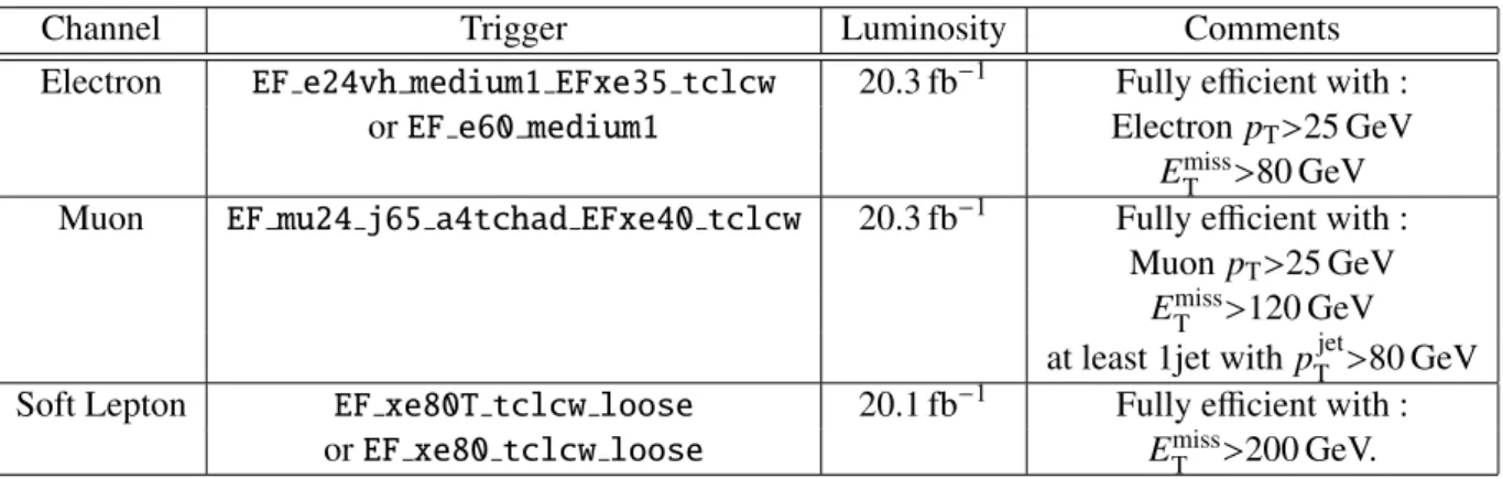
3.8 Triggers . . . 43

4 Data and Monte Carlo simulation 47 4.1 Data samples . . . 47

4.1.1 Luminosity measurement . . . 47

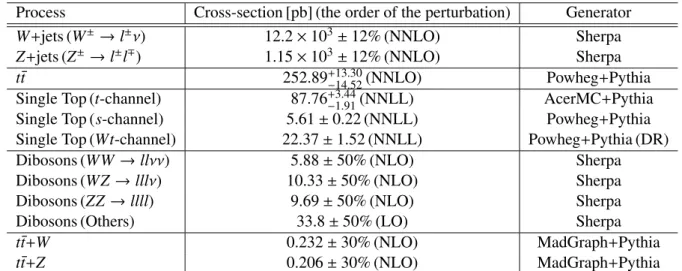
4.2 The Standard Model samples . . . 48

4.2.1 Standard Model processes . . . 49

4.3 Signal samples . . . 51

4.3.1 Signal models . . . 51

4.3.2 MSUGRA/CMSSM model . . . 51

4.3.3 Simplified models . . . 52

5 Signal Region optimization 55 5.1 Event topology . . . 55

5.1.1 Signals . . . 55

5.1.2 W+jets . . . 55

5.1.3 t¯t . . . 56

5.1.4 Kinematic variables for signal region optimization . . . 56

5.2 Signal Region Optimization . . . 59

6 Background estimation 65 6.1 Multi-jet background . . . 65

6.2 W+jet and t¯t backgrounds . . . 65

6.2.1 Control Regions . . . 65

6.2.2 Validation Regions . . . 66

6.2.3 t¯t correction . . . 66

6.2.4 W+jets correction . . . 75

6.2.5 Fitting in the Control Regions . . . 78

6.2.6 Data/MC comparison . . . 79

6.3 Other backgrounds . . . 79

7 Uncertainties 81 7.1 Instrumental uncertainties . . . 81

7.1.1 Jet Energy Scale (JES) uncertainty . . . 81

7.1.2 Jet Energy Resolution (JER) uncertainty . . . 81

7.1.3 Lepton energy scale, resolution, and trigger/reconstruction efficiency uncertainties 82 7.1.4 Emiss T resolution uncertainties . . . 82

7.1.5 Pile-up uncertainties . . . 82

(5)

7.2 Theoretical uncertainties . . . 83 7.2.1 t¯t . . . 83 7.2.2 W+jets . . . 83 7.2.3 Single Top . . . 84 7.2.4 Z+jets . . . 84 7.2.5 t¯t+V . . . 84 7.2.6 Dibosons . . . 85 7.2.7 QCD multi-jet . . . 85 7.3 Signal uncertainties . . . 85 7.3.1 Cross-section uncertainty . . . 85 7.3.2 Acceptance uncertainty . . . 85 8 Results 88 8.1 Un-blinding the Signal Regions . . . 88

8.2 Limit calculation . . . 92 8.3 Interpretation . . . 94 8.3.1 MSUGRA/CMSSM . . . 94 8.3.2 Simplified models . . . 96 8.4 Discussion . . . 100 9 Conclusion 102 Bibliography 105 A Higgs mechanism 111 A.1 Electroweak theory . . . 111

A.2 Gauge theory . . . 111

A.3 Higgs mechanism . . . 112

B Details of Signal Region optimization 115 B.1 Setup . . . 115

B.2 Results . . . 117

C Matrix-Method 121 C.1 Lepton misidentification rate . . . 121

C.2 Lepton identification efficiency . . . 122

C.3 Validation . . . 123

D Fit results for the Control Regions 126 E Fit results for the Validation Regions 128 F Emiss T and mTfor the events in the SRs 132 G Fit results for the Signal Regions 135 H Profile-likelihood and CLs 138 H.1 Likelihood . . . 138

H.2 Profile-likelihood . . . 138

(6)

H.3 CLsmethod . . . 140

I Tile Calorimeter calibration using scrapping muon 142 I.1 Introduction . . . 142

I.1.1 Tile calorimeter . . . 142

I.1.2 Muon spectrometer system . . . 142

I.1.3 Trigger system . . . 143

I.1.4 Scraping beam . . . 143

I.2 Data analysis . . . 143

I.2.1 Muon track selection criteria . . . 143

I.2.2 Monte Carlo simulation . . . 144

I.2.3 Calorimeter response and further selection criteria . . . 144

I.3 Results . . . 146

I.3.1 Uniformity of calorimeter cell response . . . 146

I.3.2 Inter-calibration of radial layers . . . 146

(7)

1 The Standard Model and Supersymmetry

1.1 Introduction

The Standard Model (SM) is a quite successful model to describe the phenomena below the electroweak energy scale of O(100) GeV with great accuracy. On the other hand, once we consider higher energy up to the Grand Unified Theory (GUT, ΛGUT∼1016GeV) or The Planck scale (Mpl=1.22 × 1019GeV), there arise some problems the SM cannot explain.

One natural question is “why the electroweak energy scale and the GUT or Planck scales are so separated by a significant order?”, which is called “hierarchy problem”. The hierarchy problem gives rise to a problem on the Higgs mass, whose bare mass receives large radiative corrections of an order of the fundamental scale. To yield the physical Higgs mass at the electroweak scale, a large degree of cancellation between bare mass and quantum corrections is needed (naturalness problem). The long-sought Higgs boson, the final missing ingredient in the Standard Model, was discovered at the LHC in 2012 [1]. The mass of the Higgs boson was measured to be ∼126 GeV, which is an interesting challenge to naturalness and the discovery of supersymmetric particles at the LHC. The WMAP [2] experiment made a valuable measurement of the fraction of ingredients of the universe. The results suggest that more than 85 % of the total matter in the universe is made of “Dark Matter” (DM), for which the Standard Model does not have an appropriate candidate. Gravity is also a problem which is not described within the framework of the SM. Supersymmetry is one of the solutions aiming to solve the problems mentioned above. The brilliant solution of supersymmetry will be discussed in Section 1.4 after introducing the SM in the next Section.

1.2 The Standard Model

The Standard Model consists of two theories: electroweak theory and Quantum ChromoDynamics (QCD). Electroweak theory is particularly interesting because it introduces the Higgs mechanism, which also plays an important role in supersymmetry theories. We start from introducing elementary particles and forces in the Standard Model, then describe electroweak theory. QCD theory is explained later mainly from the experimental aspect.

1.2.1 Elementary particles in the Standard Model

In the framework of the Standard Model, matter consists of quarks and leptons, which are collectively-referred to as fermions. There are six types of quarks (up, down, charm, strange, top and bottom) and six leptons (electron, muon, tau and their paired neutrinos). As shown in Fig. 1, they are classified into three groups, called generations. An anti-particle accompanies for each fermion with the same mass but the opposite quantum numbers, such as charge. All fermions have spin1

2.

There are the particles which intermediates forces between fermions, which are called gauge bosons. A photon conveys the electromagnetic force, W±_{and Z}0_{bosons intermediate the weak force and a gluon} conveys the strong force. All these bosons have spin 1. The remaining force, gravity, is not included in the framework of the Standard Model.

1.2.2 Electroweak theory

Detailed description of electroweak theory and the Higgs mechanism are documented in Appendix A, so only a simple overview and several important notations are introduced here.

The weak force couples through weak isospin, which obeys SU(2) symmetry (to avoid confusion, we add a subscript L in the following). The left-handed fermions are put into SU(2)Ldoublets, such as

(8)

! uL dL " and ! νL eL "

. Here the subscript means that the fermions are left-handed. The doublets are denoted by capital letters, such as L for leptons and Q for quarks. A right-handed fermion forms SU(2)Lsinglet and represented by a small letter with subscript R, for example, eR(electron), uR(up quark). Then we introduce U(1) symmetry, which is proportional to Hypercharge Y. Gauge theory give birth to electro-magnetic and the weak interactions at the same time from U(1)Y×SU(2)Lsymmetry. In the framework of gauge theory, the gauge bosons are prohibited to have explicit mass terms, which is opposed to ex-perimental results. This problem is solved by the Higgs mechanism. The Higgs mechanism introduces a SU(2)L complex scalar doublet φ with an unstable potential. As a result of Spontaneous Symmetry Breaking (SSB), a new stable vacuum is chosen where the massive bosons arise. The expectation value of the Higgs field after SSB 'φ( is called Vacuum Expectation Value or VEV. Fermion masses are also explained in gauge theory through Yukawa coupling constant y.

Figure 1: Particles in the Standard Model.

1.2.3 QCD

Quantum Chromo Dynamics (QCD) describes the strong interactions of quarks and gluinos. The theory has “Chromo” in its name because the theory is based on SU(3)C symmetry and fundamental represen-tation3 seems to behave like three colors. A quark (anti-quark) obeys 3 (¯3) representation. A 8 represen-tation generated in3 ⊗ ¯3 = 8 ⊕ 1 is assigned to a gluon. Another difficulty of QCD is that the strength of its coupling constant αS is too strong to perform perturbative calculations. As a result, first or second order perturbation doesn’t give sufficient accuracy, which weakens the prediction power.

A complete overview of QCD goes far beyond the scope of this thesis, therefore, only important conclusions necessary in the analysis are summarized.

Asymptotic freedom :

In renormalization group theory, the running of coupling constant is evaluated by β-function. In the lowest non-trivial order, β-function for SU(3) theory with the number of generation ngen is

(9)

given as β1(α) = α 2 2π # −11 + ngen₃ $, (1)

where α represents the coupling constant, α = g2

4π. For QCD, ngen is 3, which results in a negative value for the β-function. A negative β-function means that the coupling constant becomes weaker at higher energy. This feature makes perturbative calculations possible in hard collisions at the LHC energy scale, while the calculations of low energy phenomenon around ΛQCD ∼ O(1) GeV become difficult, because the coupling constant diverges near ΛQCD, which breaks the perturba-tion. This behavior is problematic for jet shower simulation since jet shower is made up of many productions of light hadrons at the energy scale of O(1) GeV. To cope with the problem, Monte Carlo generators stop jet evolution at some energy scale and the existing quarks are forced to be changed into hadrons. This technical trick is called “Hadronization”.

Even at high energy, the coupling constant αS depends strongly on the energy scale compared with weak or electromagnetic coupling constants. As a result, the choice of the energy scale at which αS is evaluated becomes important. In Monte Carlo simulation, the energy scale, called renormalization scale, is determined by an empirical formula. Therefore impact of the choice is evaluated by varying the energy scale and taken into the uncertainty.

Confinement :

QCD predicts a very strong forces between two colored particles. Contrary to electromagnetic forces, it becomes stronger when they are separated farther. As a result of this behavior, there exists a distance at which the potential energy exceeds quark masses, and beyond the distance, creation of a new particle pair is favored in the light of the total energy. The distance is smaller than the diameter of proton, so it is impossible to see an isolated colored particle, which is often said as colored particles are “confined”.

As a result, a few number of quarks and gluinos produced in a collision consequently pair-create a lot of particles as they get separated, forming a shower-shape jet. This process is called “fragmen-tation”.

1.3 Problems of the Standard Model

Although the Standard Model describes a wide range of phenomena, there exist several exceptions which cannot be explained in the Standard Model. The followings are such interesting phenomena. They’re important because they might lead to the theories beyond the Standard Model.

1.3.1 Grand unification

In the grand unification theory, electromagnetic, weak and strong forces are thought to stem out from one force at the GUT scale. If it is correct, the coupling constants for these three forces should be the same strength at the GUT scale. In renormalization theory, the energy dependence of coupling constant αi is evaluated by 1 αi(Q)2 − 1 αi(Q0)2 =− bi 2πln ! Q Q0 " , (2)

where Q0is the energy scale at which the coupling constant αiis measured (usually mZis chosen) and Q is the energy scale at which αiis evaluated. In the Standard Model, biis

bSM i =    b1 b2 b3    =    0 −223 −11    + ngen    4 3 4 3 4 3    + nHiggs    1 10 1 6 0   , (3)

(10)

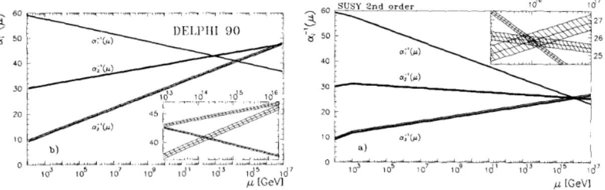
where ngen is the number of generations and nHiggsis the number of Higgs doublets, which are 3 and 1, respectively. Parameters in the parentheses are the function of number of particles appearing in loop calculations. The running of coupling constants are evaluated as plotted in Fig. 2 (left). The three lines do not intersect at one point.

On the other hand, in Minimal Supersymmetric Standard Model (MSSM), which will be introduced later, the coefficients biare modified because of newly introduced particles. bi, then, becomes,

bMSSM_i =    b1 b2 b3    =    0 −6 −9    + ngen    2 2 2    + nHiggs    3 10 1 2 0   . (4)

Note that the number of Higgs fields nHiggsis 2 in MSSM. If supersymmetry exists at the mass scale of around O(1) TeV, the three coupling constants cross around Q = O(1016_{) GeV and the grand unification} occurs as shown in Fig. 2 (right).

Figure 2: First order evolution of the tree coupling constants in the Standard Model using MZ and αS(MZ) from DELPHI data (left) and the second order evolution of the tree coupling constants in MSSM assuming SUSY mass scale MSUSYof around 1 TeV (right) [3].

1.3.2 Hierarchy problem

Masses of the SM particles are all below the electromagnetic scale, i.e. O(100) GeV, while the Planck scale is MPl ∼ 1016GeV, where gravity finally becomes as strong as the other three forces. The unnatural splitting between these energy scales are called “hierarchy problem”.

Another problem, which is also called “hierarchy problem”, occurs for the Higgs mass. In the lead-ing order, the Higgs mass is O(100) GeV (see Appendix A.3), however, once we include higher order corrections, the one-loop diagram containing a Dirac fermion f with mass mf, shown in Fig. 3 (left) also contributes. If the Higgs field couples to f through a term −λfH ¯ff , then the Feynman diagram in Fig. 3 (left) yields a correction of

∆m2

H =−|λf| 2

8π2Λ2UV+ ..., (5)

where ∆UV is ultraviolet energy cutoff used to regulate the loop integral, or it can be interpreted as the energy scale to which the SM is valid. If there is no new physics beyond the SM up to the Planck scale, then the Higgs mass diverges quadratically.

Let’s assume a heavy complex scalar particle S with mass mS that couples to the Higgs through a term −λS|H|2|S |2, the Feynman diagram in Fig. 3 (right) gives a correction of

∆m2_H= λS

(11)

As shown later, two scalar particles are newly introduced for each of the SM fermion in the supersym-metry framework. If these scalar particles have coupling constants satisfying λS = |λf|2, the first terms of Eq. 5 and Eq. 6 cancel each other and the problematic quadrature divergence does not occur any more. This cancellation mechanism is the primary motivation of introducing supersymmetry.

1.3.3 Dark matter

WMAP [2] measured the contents of the universe in a great accuracy: Ωbh2 = 0.0227 ± 0.0006, Ωcdmh2 = 0.110 ± 0.006,

ΩΛ = 0.74 ± 0.03,

(7) where h is a dimensionless parameter defined from the Hubble constant H0,

H0=100 h km s−1Mpc−1. (8)

All the values on the right-hand-side in Eq. 7 are the fractions with respect to the critical density of the universe ρc, which is

ρcc2=5.4 ± 0.5 GeV · m−3. (9)

Ωbh2is the fraction of Baryonic matter, Ωcdmh2is the fraction of cold Dark Matter and ΩΛrepresents the dark energy. The coldness (or slowness) of dark matter is important for formation of complex structure in the universe, such as galaxy. Assuming a hot dark matter with a relativistic speed, the structure gets smoothed and no star is formed. The dark matter should have the following properties:

• To explain the contents of current universe, dark matter should be stable over the lifetime of the universe.

• The charge of dark matter should be zero, therefore electromagnetic force cannot or only weakly interact with dark matter.

• To be a cold dark matter, it should be heavy. A quantitative limit comes from a comparison with the mass and the energy scale at which dark matter decoupled from heat-equilibrium in the early universe.

There’s no particle which satisfies above conditions in the framework of the Standard Model.

Weakly Interacting Massive Particles (WIMPs) is one of the candidates. WIMPs have masses roughly between 10 GeV and a few TeV, and an interaction cross-sections of the weak force. As shown later, the lightest supersymmetry particle (LSP) cannot decay further in R-parity conserving supersymmetry models and becomes a good dark matter candidate satisfying above requirements.

(12)

H

f

S

H

Figure 3: Example diagrams showing 1-loop radiative corrections which contribute to mh. The loop of a Dirac fermion f (left) with a coupling constant λf and the one of a scalar particle S (right) with a coupling constant λS.

(13)

1.4 Supersymmetry

As discussed in the previous section, the Standard Model contains some problems and there must be a new physics beyond the SM. Pursuing the theory of everything, many theorists have proposed solutions in the last several decades. Supersymmetry introduces “superpartners” of the SM particles which have different spin by 1

2. Since fermions and bosons have spin12 and spin 0, respectively, supersymmetry is often referred to as symmetry between fermion and boson.

There exist several supersymmetry models with different particle contents. We focus on the simplest model, Minimal Supersymmetric Standard Model (MSSM), which contains the minimal extension of the Standard Model particles.

1.4.1 SUSY breaking

Although the basic concept of supersymmetry is simple, recalling the fact that the superpartner with exact the same mass has not yet been observed, supersymmetry must be “broken” in a sense that supersym-metric particles are much heavier than the SM partners. We see how the SUSY breaking is introduced in the MSSM framework below1_.

We start from introducing the most general form of SUSY breaking Lagrangian [4], which is LMSSM

soft = 12

+

M3˜g˜g + M2W ˜˜W + M1˜B ˜B + c.c., −+˜¯uauQH˜ u− ˜¯dadQH˜ d− ˜¯eae˜LHd+c.c., − ˜Q†_m2

˜

QQ − ˜L˜ †m2˜L˜L − ˜¯um2˜¯u˜¯u†− ˜¯dm2_˜¯d˜¯d†− ˜¯em2˜¯e˜¯e† −m2HuHu∗Hu− m

2

HdHd∗Hd− (bHuHd+c.c.)

. (10)

The terms in the Lagrangian are chosen so that the resultant SUSY breaking does not introduce the quadrature divergence again. The first line gives masses to the superpartners of gauge bosons. M3, M2 and M1correspond to the masses of gluino ˜g, wino ˜W and bino ˜B, respectively. The second line contains (scalar)3 _{type interactions (trilinear coupling). ˜¯u, ˜¯d, ˜¯e are the vector of right-handed up-type squarks,} down-type squarks and sleptons. Each component of the vector represents a particle in three generations.

˜

Q, ˜L are similar vectors but of left-handed particles, each of which is a weak isospin doublet as in Eq. 108. Hu,Hd are the Higgs potentials which couple to up-type and down-type fermions. Finally,au,ad,ae are complex 3 × 3 matrices in family space with dimension of mass. These terms resemble the fermion mass term in Eq.108 and actually the terms are in one-to-one correspondence with the Yukawa couplings,

au =Au0yu, ad= Ad0yd, ae =Ae0ye, (11)

where, yX is called Yukawa matrix in which the Yukawa couplings are contained as the components. The third line consists of squark and slepton mass terms. Each ofm2

˜

Q,m2˜L,m2˜¯u,m2˜¯d,m2˜¯e is a 3 × 3 matrix in family space that can have complex entries. However, from the experimental limits on the flavor-changing neutral current and CP-violation, the squark and slepton mass matrices are required to be flavor-blinded, which is realized when the mass matrices are proportional to the identity matrix1 before renormalization group evolution:

m2 ˜ Q=m2Q˜1, m2˜¯u=m2˜¯u1, m2_˜¯d=m2_˜¯d1, m2 ˜L=m2˜L1, m2˜¯e =m2˜¯e1. (12) Finally, in the last line of Eq. 10 we have supersymmetry breaking contributions to the Higgs potential. m2

Hu,m

2

Hd are the contributions to the up-type and down-type Higgs masses.

1_{The discussion is closely related to the content of the next section, so one should refer the Section 1.4.2 when an undefined}

(14)

The original SUSY breaking Lagrangian contains many free parameters, especially as the compo-nents of matrices. However, introducing the assumptions such as Eq. 11 and Eq. 12, 124 parameters in the original Lagrangian are reduced to a few parameters.

1.4.2 Particles in MSSM

Next, we look into the particles introduced in MSSM and their properties. Figure 4 illustrates the corre-spondence between the SM particles and their superpartners in MSSM.

Figure 4: Illustrations of the SM particles and their corresponding superpartners in the framework of MSSM.

Higgs and Higgsino :

In the MSSM framework, two Higgs doublets with weak hypercharges of Y = +1/2 and Y = −1/2 are introduced. The former one, denoted as Hu, gives masses to up-type fermions, while the latter one, Hd, couples to down-type fermions. Each of them is composed of neutral and charged components, Hu = ! H+ u H0 u " , Hd = ! H0 d H− d " . (13)

Inserting the components into the SUSY Lagrangian, we obtain a potential related to the Higgs boson V = (|µ|2+m2_H_u)(|H_u0|2+|H+_u|2) + (|µ|2+m2_H_d)(|H_d0|2+|H_d+|2) (14) + |b(H_u+H_d−− H_u0H_d0+c.c.| (15) + 1 8(g2+ g+2))(|Hu0|2+|Hu+|2− |Hd0|2− |Hd0|2− |H−d|2)2 (16) + 1 2g2|Hu+Hd0∗+Hu0Hd−∗|2, (17)

(15)

where g, g+_{are the gauge coupling constants and the terms proportional to µ come from the Higgs} interaction terms in the SUSY Lagrangian. We perform the same calculation of SSB as in the Higgs mechanism in the Standard Model, i.e. find the minimum of potential V and expand the potential about the minimum. Using SU(2)L and U(1)Y symmetries, we can set Hu+ = Hd− = 0. Also, the vacuum expectation values of the two remaining Higgs fields, 'H0

u( and 'Hd0(, can be set to real and positive. We require that the VEVs are compatible with the observed phenomenology of electroweak symmetry breaking. Let us write

vu ='H_u0(, vd='H_d0(. (18)

Then, the quadrature sum of these two terms corresponds to v in the Standard Model,

v2= v2_u+ v2_d. (19)

The ratio of the VEVs is written as

tan β = vu

vd. (20)

The original Higgs doublets have eight freedom in total. Three of them are eaten by three elec-troweak bosons and five freedoms remain as physical Higgs fields. They consist of two CP-even natural scalar bosons h0 _{and H}0_{, one CP-odd natural scalar boson A}0_{and a charge +1 scalar} bo-son H+_{and its conjugate charge -1 scalar boson H}−_{. The mass of each Higgs field is given as}

m2_A0 = 2|µ|2+m2Hu +m 2 Hd, (21) m2_h0_,H0 = 1 2   m2A0 +m2Z∓ -+ m2 A0− m2Z ,2 +4m2_Zm2_A₀sin2(2β)    , (22) m2_H± = m2_A0 +m2W. (23)

|µ| is obtained by the following relation: m2 Z = |m2Hd − m 2 Hu| . 1 − sin2(2β) − m 2 Hu − m 2 Hd − 2|µ| 2_. ₍₂₄₎

Note that these Higgs masses are obtained at tree-level calculations. The radiative correction to the Higgs mass will be discussed in Section 1.4.5.

The superpartners of the Higgs bosons are called Higgsinos. The superpartners for the neutral components are denoted as ˜Hu and ˜Hd, and those of the charged components are ˜H+ and ˜H−, respectively. The mass of Higgsinos is given by µ.

Gluino :

The superpartners of gluon is called gluino ˜g. The mass of gluinos is represented as M3as shown in Eq 10.

Wino and Bino :

The superpartners of electroweak gauge bosons are called wino ˜W and bino ˜B (they are collectively-referred to as electroweak gauginos). The masses of winos and bino are given by M2 and M1, respectively.

The higgsinos and electroweak gauginos mix with each other because of the effects of electroweak symmetry breaking. Neutral higgsinos and neutral gauginos combine to form four mass eigenstates

(16)

called neutralinos. In the gauge-eigenstates basis Ψ0 ₌+ ˜B, ˜W0_{, ˜}_H0 d, ˜Hu0

,

, the neutralino mass part of the Lagrangian is Lneutralino mass = 1 2(Ψ0)TM˜NΨ0+c.c., (25) where M˜N =     M1 0 −cβsWmZ sβsWmZ 0 M2 cβcWmZ −sβcWmZ −cβsWmZ −cβcWmZ 0 −µ sβsWmZ −sβcWmZ −µ 0    . (26)

Here we introduced abbreviations: sW =sin θW,cW =cos θW, sβ=sin β and cβ=cos β.

The charged Higgsinos and winos mix in a similar way to form two mass eigenstates with charge ±1, which are called charginos. In the gauge-eigenstate basis Ψ±₌_{( ˜}_W±_{, ˜}_H±

u/d), the chargino mass terms in the Lagrangian are

Lchargino mass=−1 2(Ψ±)TM˜NΨ±+c.c. (27) with M_˜N = ! M2 √2sβmW √ 2sβmW µ " . (28)

We denote the neutralino and chargino mass eigenstates as ˜χ0

i (i = 1, 2, 3, 4) and ˜χ±i (i = 1, 2). The labels are assigned so that m_˜χ0

1 <m˜χ02 <m˜χ03 <m˜χ04 and m˜χ±1 <m˜χ±2.

Squark and Slepton :

Squarks ˜q are the superpartners of quarks. They have the same quantum numbers of the corre-sponding quarks except for spin and mass. They behave in the same way as their partners under gauge interactions. The superpartners of left-handed and right-handed quarks are written as ˜qLand ˜qR. However, since sparticles do not have helicities, the handedness does not refer to its helicity but just specifies its quantum numbers. So, for example, only a left-handed squark ˜qL couples to W bosons while a right-handed squark ˜qR doesn’t. With this notation, gauge interactions are consistent with their SM partners.

Similarly, sleptons ˜l are the superpartners of leptons. These superparticles also have the same quantum numbers as their SM partners except for spin and mass.

The masses of the first and second generation squarks and sleptons are calculated as follow assum-ing they have the same mass m0at the GUT scale,

m2 ˜dL =m 2 0 +K3 +K2 +361K1 +∆˜dL, m2 ˜uL =m 2 0 +K3 +K2 +361K1 +∆˜uL, m2 ˜uR =m 2 0 +K3 +49K1 +∆˜uR, m2 ˜dR =m 2 0 +K3 +19K1 +∆˜dR, m2 ˜eL =m 2 0 + +K2 +14K1 +∆˜eL, m2 ˜νe =m 2 0 + +K2 +14K1 +∆˜ν, m2 ˜eR =m 2 0 + +K1 +∆˜eR, (29)

K3, K2 and K1 represent the contributions obtained during the renormalization group evolution, which are related to SU(3)C, SU(2)L and U(1)Y forces, respectively. Since left-handed squarks, ˜dL,˜uL, feel all three forces, all the term contributes to their masses. Right-handed squarks, ˜uR, ˜dR, do not couple to SU(2)Lforce, therefore K2term doesn’t contribute. Left-handed sleptons, ˜uR, ˜dR,

(17)

do not interact with SU(3)C as they don’t have color charges. Right-handed slepton, ˜eR, is the lightest among these particles since it feels only U(1)Y force through hypercharge Y.

The last term ∆X represents a small contribution from the electroweak symmetry breaking [4]. We focus on the heavy particles for which this contribution is negligible.

Assuming the coupling constant unification occurs at Q0 =2 × 1016GeV and fermion masses are unified at that energy scale, the following values are obtained at the electroweak scale:

K1∼ 0.15m2_1/2, K2∼ 0.5m2_1/2, K3∼ (4.5 − 6.5)m2_1/2, (30) where m1/2is the unified mass of gauginos at the GUT scale.

Due to strong Yukawa couplings, masses of third generation squarks and sleptons take different forms. Here we take stop ˜t for example but the same discussion hold for sbottom and stau as well. Left- and right-handed stops are mixed by the interactions with the Higgs potential and the soft breaking term. We consider the terms which contributes to the following mass Lagrangian:

Lstop masses =−+˜tL∗ ˜tR∗ , m2 ˜t! ˜t_˜tL_R " . (31)

First, a contribution of the form y2

tH0∗u ˜t∗L˜tLand y2tHu0∗˜t∗R˜tR(the diagrams are shown in Fig. 5) con-tribute to the diagonal terms. At the VEV, ytHu is equal to top mass, therefore this contribution gives a mass term proportional to the top mass mt. Second, the diagram shown in Fig. 6 contributes to the off-diagonal term. This interaction is represented as −µ∗_y_t_{(v cos β)˜t}∗

R˜tL+c.c.. The final con-tribution comes from the soft breaking term which is represented as at(v sin β)˜tL˜t∗_R+c.c.. This term contributes to the off-diagonal term as it mixes left- and right-handed stops.

Adding up these terms, we obtain the mass matrix of stopsm2 ˜t, m2 ˜t = ! _m2 Q3+m 2

t + ∆˜uL v(a∗t sin β − µytcos β)

v(a∗

t sin β − µytcos β) m2_¯u₃ +m2_t + ∆˜uR

"

. (32)

In a similar way, one can obtain the mass matrix of sbottom in the gauge-eigenstate basis of (˜bL, ˜bR) with the right-handed squark mass of

m2

˜b =



 m2Q3 + ∆˜dL v(a∗bcos β − µybsin β)

v(a∗

bcos β − µ∗ybsin β) m2¯d3+ ∆˜dR



, (33)

and the stau mass matrix in the gauge-eigenstate basis of (˜τL,˜τR) is m2˜τ =

! _m2

L3 + ∆˜eL v(a∗τcos β − µyτsin β)

v(a∗

τcos β − µ∗yτsin β) m2¯e3 + ∆˜eR

"

. (34)

The mass eigenstates are denoted as ˜t1, ˜t2, ˜b1, ˜b2, and ˜τ1,˜τ2. The subscripts are defined so that m˜X1 <m˜X2. The masses of third generation fermions at the electroweak scale, mQ3, m¯u3, m¯d3, mL3,

and m¯e3, are summarized in Eq. (6.5.41)-(6.5.45) in Ref. [4].

1.4.3 R-parity

In MSSM, one needs to introduce a new symmetry in order to forbid the term which induces the baryon and lepton number violations. It is called R-parity PRand written as

(18)

H0 u Hu0∗ ˜tL ˜t∗L H0 u Hu0∗ ˜tR ˜t∗R

Figure 5: Interactions with the form of (scalar)4_{. The coupling constant is proportional to y}2 t.

H0∗

d

˜tL ˜t∗R

Figure 6: Interaction with the form of (scalar)3_{. The coupling constant is proportional to µ}∗_y_t_.

where B and L are the baryon and lepton numbers, and s denotes the spin. PR takes +1 for the SM particles and −1 for the SUSY partners. Models that violate R-parity are also possible if the resultant violations are well below experimental limits, but in this thesis only the R-parity conserving models are considered. As a result of R-parity conservation, SUSY particles must be produced in pairs and they decay to stable Lightest SUSY Particles (LSP).

1.4.4 Minimal supergravity model

The original 124 free parameters in the SUSY breaking Lagrangian are reduced down to a few parameters by the assumptions from experimental requirements such as Eq. 11 and Eq. 12. The number of parameters can be further reduced by introducing SUSY-breaking models.

The breaking is assumed to originate in the hidden sector, which is the collection of unobserved hy-pothetical particles that do not directly interact via the Standard Model gauge bosons, and the breaking ef-fect is transferred to the MSSM sector by a specific mechanism. In Minimal Supergravity model (MSUGRA) or Constrained Supersymmetry model (CMSSM), gravity is thought to be the messenger that mediates the breaking. The parameters in MSUGRA/CMSSM model is reduced to 4 and one sign, which makes the model highly predictive.

m0: All masses of squarks and sleptons are assumed to be universal at the GUT scale, which is repre-sented by m0.

m1/2: All masses of gauginos are assumed to be universal at the GUT scale, which is represented by m1/2. The following relationship holds for gaugino masses,

M1 5 3g+2 = M2 g2 = M3 g2_S =m1/2. (36)

(19)

At the electroweak scale, they are

M1∼ 0.4m1/2, M2∼ 0.8m1/2, M3∼ 2.4m1/2.

(37) A0: All trilinear couplings (Eq. 11) are common in this model.

tan β: The ratio of VEVs of two Higgs bosons as defined in Eq. 20. sign(µ): The sign of µ. The absolute value is determined through Eq. 24.

In most of the parameter space, there are two possible LSP candidates: ˜χ0

1 and ˜τ±1. However, ˜τ±1 is usually forbidden as LSP should be neutral to be a dark matter candidate.

1.4.5 Discovery of the Higgs boson

The primary motivation of supersymmetry is to solve the quadrature divergence of the Higgs mass. This, in turn, sets limits on SUSY parameters [5]. Considering the recent results of the Higgs decay branches [6], the light neutral Higgs h0_{seems to have quite the same properties of the SM Higgs boson,} which happens when h0_{is much lighter than the other Higgs particles. This configuration is referred to} as “decoupling limit”. In this limit, the Higgs mass with one-loop order correction is written as

m2 h∼ m2Zcos22β +_(4π)3 ₂m 4 t v2   ln m2 ˜t m2 t + X 2 t m2 ˜t   1 − X 2 t 12m2 ˜t       , (38)

where Xt = At − µ cot β, which is the off-diagonal term of stop mass matrix in Eq. 32. Figure 7 shows the contours of mhas a function of stop mass m˜tand the stop mixing parameter Xt for tan β = 20. The red/blue bands show the Higgs mass range mh=124-126 GeV obtained by two different programs. The dotted lines show the degree of fine-tuning ∆, which is defined as the maximum sensitivity to fundamental parameters pi, ∆_{≡ max} i 55 55 55 5 ∂ln m2_h ∂pi 55 55 55 5. (39)

The smallest fine-tuning is obtained when |Xt| = √6m˜t, which is referred to as “maximal mixing”. The parameters of MSUGRA/CMSSM sample used in the analysis are chosen so that this maximal mixing is realized. In this configuration, one of the stop masses becomes 20-30% lighter than the masses without mixing. As a result, stops are more likely to appear in decay chains, which increase the complexity of events.

The Higgs mass is also affected by a gluino mass through 2-loop order corrections [7, 8], which sets an limit on a gluino mass M3:

M3<_∼900 GeV sin β!log(Λ/TeV) 3 "−1 # _m_h 120 GeV $ ! ∆−1 20 % "−12 , (40)

where Λ denotes the SUSY breaking scale. Allowing 10% fine-tuning, one finds the gluino mass should be below about 1.3 TeV. Although the limit varies depending on the fine-tuning condition, we safely expect that the gluino mass lies at O(1) TeV and inside the LHC energy scale.

(20)

Figure 7: Contours of mh in MSSM as a function of a common stop mass m˜t and the stop maxing parameter Xtfor tan β = 20. The red/blue bands show the Higgs mass range mh=124-126 GeV obtained by two different programs. The dotted lines show the degree of “fine-tuning”. This plot is cited from Ref. [5].

(21)

2 LHC and ATLAS detector

2.1 Large Hadron Collider

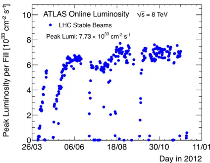
The Large Hadron Collider (LHC) [9] was constructed to collide two proton beams with an unprece-dented center-of-mass energy of 14 TeV and a luminosity of 1034_cm−2_s−1_{aiming at an investigation of} electroweak symmetry breaking and searches for the Higgs boson as well as physics beyond the Standard Model. During the data taking period in 2012, the accelerator was operating at a center-of-mass energy of 8 TeV with a peak luminosity of 7.73 × 1033_cm−2_s−1_{. Figure 8 shows the peak luminosity recorded} by ATLAS in 2012.

The beam circulating in the LHC ring is clustered to small chunks, called bunch, with a few cm in length and the transverse size of O(10) µm, containing approximately 1 × 1011 _{protons per bunch. The} bunches make collisions at the center of the detectors every 50 ns, which is twice lower rate than the original design. This is due to the beam instability observed during the run and will be cured in the next data taking phase, giving the designed collision rate of 25 ns or 40 MHz. Table 1 summarizes the proton beam parameters of the LHC.

Designed Parameters Current Parameters

Proton Energy [GeV] 7000 4000

Number of Protons in a bunch 1.15 × 1011 _{1 × 10}11

Number of Bunches in the ring 2808 1380

Peak luminosity [cm−2_sec−1_] _{1.0 × 10}34 _{7.73 × 10}33

Bunch spacing [ns] 25 50

Table 1: Designed LHC beam parameters and the ones in 2012 data taking period.

Day in 2012 26/03 06/06 18/08 30/10 11/01 ] -1 s -2 cm 33

Peak Luminosity per Fill [10

0 2 4 6 8

10 ATLAS Online Luminosity s = 8 TeV

LHC Stable Beams -1 s -2 cm 33 10 × Peak Lumi: 7.73

Figure 8: Peak luminosity recorded by the ATLAS detector per day in 2012.

The LHC is installed in the tunnel where LEP machine was originally placed. Total length of the tunnel is 26.7 km and the whole part lies about 100 m below the ground surface. The LHC uses

(22)

super-conducting magnets to bend 4 TeV beams. The original proton is produced from hydrogen gas by strip-ping the electron, then the proton is accelerated by LINAC2 to 50 MeV. The proton is fed to Proton Syn-chrotron Booster (BOOSTER) to obtain 1.4 GeV, and passed to the following accelerator, called Proton Synchrotron (PS), which accelerates the proton to 450 GeV, and finally, the 450 GeV proton is injected to the LHC. The LHC accelerates the proton to the target energy of the experiment.

There are four big experiments running in the LHC. ATLAS and CMS [10] are general-purpose detec-tors designed for studying Higgs boson and the physics beyond standard Model. LHCb [11] experiment studies B-physics, and ALICE [12] is dedicated to heavy ion collisions. Figure 9 shows the schematic overview of the LHC and four experiments.

(23)

2.2 ATLAS detector

The ATLAS2 _{experiment [13, 14, 15] is a general-purpose detector placed at the LHC. It is designed to} study various types of physics signatures, which allows to discover the Higgs boson, extra dimensions and also supersymmetry. As opposed to CMS detector, which is also targeting new physics, the ALTAS detector is designed as huge as possible so as to measure the tracks precisely by making the most of the detector length or to minimize the escaping shower energy from the calorimeter. As a result, the ATLAS detector is 44 m along the beam axis and 22 m in diameter.

2.2.1 Coordinate system

The x-axis is defined as the direction of the center of LHC ring, and the y-axis points to the opposite direction from the center of the earth. A right-handed coordinate system is used in the ATLAS, therefore the z-axis points along the beam axis. A-side is defined as the part of ATLAS detector with positive z, and C-side is the opposite. Azimuthal angle φ and polar angle θ are defined in a usual way of the right-handed coordinate, so φ is the angle around the beam axis, starting from the direction of x-axis, and θ is the polar angle from z-axis.

Pseudo-rapidity η is defined using θ

η =_{− ln tan}# θ 2 $

. (41)

Pseudo-rapidity η is an approximation of the following rapidity y at the mass-less limit y = 1 2ln ! E + pz E − pz " , (42)

where E is the energy of a given particle and pz is the transverse momentum. Here, “transverse” is defined with respect to z-axis. The distance of given two objects ∆R is often used, which is defined as the square-sum of η and φ distances,

∆R = .∆η2+ ∆φ2. (43)

2.2.2 Magnet system

The ATLAS magnet system consists of four super-conducting magnets. One solenoid magnet is im-mersed inside the detector and two toroidal magnets placed at the end-cap of A and C-sides. The last big toroidal magnet is placed outermost of the detector around the barrel.

The solenoid magnet is aligned to the beam axis and provides a 2 Tesla axial magnetic field. The magnetic field bends the tracks of charged particles in the inner detector, which allows to measure the momentum from the sagitta of tracks. A 5.8 m length solenoid is placed just inside of LAr calorimeter, which measures the energy of electron, photon and jets, so the material thickness is minimized as much as possible. A single layer coil made of Al-stabilized NbTi conductor is placed in the inner wall of the LAr calorimeter. The inner and outer diameters of the solenoid magnet is 2.46 m and 2.56 m, which corresponds to ∼0.66 radiation length at normal incidence. The return flux of the magnet is guided by the hadronic calorimeter to minimize the leakage to the muon spectrometer.

One barrel toroidal and two end-cap toroidal magnets produce toroidal magnetic field of approxi-mately 0.5 Tesla and 1 Tesla for the muon spectrometers in the barrel and in the end-cap regions, respec-tively. Figure 10 shows the schematic view of all the magnetic systems. The barrel toroid consists of eight coils encased in individual racetrack-shaped, stainless-steel vacuum vessels. The overall size of the

(24)

barrel toroid system is 25.3 m in length along the beam axis, with the inner and outer diameters of 9.4 m and 20.1 m. Each end-cap toroid consists of a single cold mass build up from eight flat, square coil units and eight keystone wedges, bolted together into a rigid structure. Both of the end-cap and barrel toroids are build up with the same materials and coil structures: pure Al-stabilized Nb/Ti/Cu conductor with a pancake-shape in section.

Figure 10: Schematic overview of the magnet system of ATLAS.

2.2.3 Tracking system

In the ATLAS detector, “tracking system” usually means the inner detectors (ID) without including out-ermost muon spectrometer (MS). The inner detectors consist of three different detectors as shown in Fig.11:

Pixel detector : The pixel detector locates the innermost layer, only 5 cm away from the beam. It con-sists of 1744 silicon pixel modules and each has pixel sensors of 50 × 400 µm along φ and z-axis. The intrinsic resolution in the barrel is 10 µm (r − φ) and 115 µm (z), and, in the end-cap disks, it is 10 µm (r − φ) and 115 µm (r).

Silicon micro-strip detector (SCT): Silicon micro-strip detector is often called as SCT, which is the abbreviation of Semiconductor Tracker. One SCT module consists of one pairs of 6.4 cm-length layers on which single-sided silicon micro-strip sensors are placed. Each micro-strip sensor layer has strip sensors with a mean pitch of 80 µm. Two strip layers are glued slightly off-aligned by ±20 m radian around the geometrical center as shown in Fig. 12, which gives the detector a sensitivity to the z-position of hits.

Transition Radiation Tracker (TRT) : TRT locates the outside of SCT system, which consists of 4 mm diameter straw tubes. The straw tube is filled with Xe gas (70 %) and some CO2, O2gas (27 % and 3 %, respectively) as quencher gas. Each straw tube has a thin wire at the center and a high voltage is applied between the wire and tube. The gaps of the straw tubes are stuffed with fibers made of polypropylene or polyethylene.

TRT detects the passage of a charged particles in two ways. One is by detecting the ionization of gas, and one is by detecting the transition radiation which is produced when a charged particle

(25)

passes the polymer fibers. Since transition radiation is emitted only from electrons and drops large energy when absorbed by gas, TRT is able to discriminate electrons from the other charged particles by setting an appropriate energy threshold.

Figure 11: Schematic overviews of tracking system. Left plot shows the cross-section and right plot gives the bird-eye view.

Figure 12: Illustration of SCT.

2.2.4 Calorimeter system

The ATLAS calorimeters cover the range of |η| < 4.9. Fine granularity electromagnetic (EM) calorime-ters are used for the precise measurement of electrons and photons. Hadron calorimecalorime-ters are made with rather coarser granularity but are sufficient for their primary purpose, jet reconstruction. Figure 13 shows the ATLAS calorimeter system and more details of Tile calorimeter are documented in Appendix I.

(26)

Figure 13: Schematic overview of ATLAS Calorimeter system.

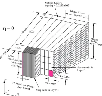
EM calorimeter EM calorimeter is divided into barrel part (|η| < 1.475) and two end-cap parts (1.375 < |η| < 3.2). EM calorimeter is Lead-LAr detector with accordion-shaped kapton electrodes and lead absorber plates over its full coverage. Figure 14 shows a sketch of EM calorimeter in the barrel region. EM calorimeter is constructed from three layers in radial direction. Additional pre-sampler detector is placed in |η| < 1.8, which consists of an active LAr layer of 1.1 cm (0.5 cm) thick in the barrel (end-cap) region. It is used to correct the energy loss in upstream material.

Tile calorimeter Tile calorimeter is placed outside of EM calorimeter in the barrel region. The central barrel part covers |η| < 1.0 and two extended barrels cover 0.8 < |η| < 1.7. Tile calorimeter collects shower energy using 14 mm thick steel plates as absorber and 3 mm thick scintillating tiles as active material. It is longitudinally segmented in three layers approximately 1.5, 4.1 and 1.8 interaction length thick for the barrel and 1.5, 2.6 and 3.3 interaction length for the extended barrel. Two sides of the scintillating tiles are read out by wavelength shifting fibers into two separate photo-multiplier tubes.

LAr hadronic end-cap calorimeter Hadronic end-cap calorimeter (HEC) consists of two independent wheels in each end-cap behind the end-cap EM calorimeter. To reduce the drop in material density in the transition part between the end-cap and the forward calorimeter around |η| = 3.1, HEC extends out to |η| = 3.2. Also HEC covers up to |η| < 1.5 in the barrel region and slightly overlaps with the barrel tile calorimeter which covers |η| < 1.7. Each wheel has four layers. The innermost layer is built from 25 mm parallel copper plates, while the outer layers use 50 mm copper plates, interleaved with 8.5 mm LAr gaps as the active medium.

LAr forward calorimeter Forward calorimeter (FCal) is integrated into the end-cap cryostat covering the range of 3.1 < |η| < 4.9. FCal is approximately 10 interaction lengths deep and consists of three modules in each end-cap. The first module is made of copper optimized for electromagnetic measurements. The other two are made of tungsten for hadronic interaction measurements. Liquid argon is used as the sensitive medium. In order to reduce the amount of neutrons reflected into the inner detector cavity, the front face of the FCal is recessed by about 1.2 m with respect to the EM calorimeter front face.

(27)

Δϕ = 0.0245 Δη = 0.025 37.5mm/8 = 4.69 mm Δη = 0.0031 Δϕ=0.0245_x4 36.8mm x4 =147.3mm Trigger Tower Trigger Tower Δϕ = 0.0982 Δη = 0.1 16X0 4.3X0 2X0 1500 mm 470 mm η ϕ η = 0

Strip cells in Layer 1

Square cells in Layer 2 1.7X0

Cells in Layer 3 Δϕ× Δη = 0.0245× 0.05

Figure 14: Expanded view of EM calorimeter. The magenta square shows the minimum unit size of EM calorimeter.

2.2.5 Muon system

The ATLAS muon system measures muon momentum using the magnetic deflection of muon tracks in the super-conducting air-core toroid magnets. Over the range of |η| < 1.4, magnetic field is provided by the barrel toroid. For 1.6 < |η| < 2.7, muon tracks are bent by the two end-cap magnets inserted into both ends of the barrel toroid. Between these regions, 1.4 < |η| < 1.6, the magnetic field is provided by a combination of barrel and end-cap magnets. Four types of muon chambers are used for the measurement of muon hit positions. Figure 15 shows the layout of the muon system.

Monitored Drift Tubes (MDT) measure the track properties precisely in the range of |η| < 2.7 (|η| < 2.0 for the innermost plane). These chambers consist of three or four layers of drift tubes, which achieve an average resolution of 80 µm per tube or about 3 µm per chamber. In the center of the detector (|η| ∼ 0), a gap in chamber coverage is left open for service. Cathode Strip Chambers (CSC), which are multi-wire proportional chambers with cathodes segmented into strips, are used in the innermost plane of 2.0 < |η| < 2.7 for additional precise track measurement. The resolution of chamber is 40 µm in the bending plane and about 5 mm in the transverse plane.

The muon trigger system consists of Resistive Plate Chambers (RPC) and Thin Gap Chambers (TGC) covering |η| < 1.05 and 1.05 < |η| < 2.4, respectively. RPC consist of three concentric cylindrical layers around the beam axis, referred to as trigger stations. Each station further consists of two independent detector layers, each measuring η and φ. TGC are multi-wire proportional chambers with the wire-to-wire distance of 1.8 mm. TGC are also used to determine azimuthal positions to complement the measurement of MDT in the bending direction.

2.2.6 Trigger system

The ATLAS experiment is designed to receive data at 40 MHz but the data acquisition system can only commit data to permanent storage at the rate of a few hundred Hz. To select “interesting” events from the large number of incoming events, trigger system are made up of three layers, Level1 (L1), Level2 (L2) and event filter (EF). L1 trigger searches for high transverse momentum muons, electrons, photons, jets, τ-leptons decaying into hadrons, large missing and total transverse energy. In each event, L1 trigger

(28)

Figure 15: Overview of Muon Spectrometer system.

defines one or more Regions-of-Interest (RoI) which is the geometrical coordinate in η and φ where an interesting feature is found. The maximum acceptable L1 rate is 75 kHz and the L1 decision must reach the front-end electronics within 2.5 µs after the bunch-crossing to tell the front-end electronics whether the event stored in the buffer should be read or discarded. L2 trigger is seeded by the RoI information provided by L1 trigger. Taking longer time to process data, L2 trigger analyses the events in more detail for further reduction of trigger rate. L2 trigger is designed to reduce the trigger rate to approximately 3.5 kHz within an event processing time of about 40 ms in average. EF trigger reduces the event rate to roughly 200 Hz, reconstructing the objects with almost the same definitions as the offline analyses and determine the event to be stored.

(29)

2.2.7 Luminosity detectors

There prepared several methods and detectors to measure the luminosity in ATLAS. LUCID (Luminosity measurement using a Cerenkov Integrating Detectors) is one of such detectors. LUCID are located on each side of the interaction point (IP) at a distance of 17 m, covering the pseudo-rapidity range of 5.6 < |η| < 6.0. LUCID are made of aluminum tubes filled with C4F10gas and surrounds the beam-pipe as shown in Fig. 16 (top left). By counting the Cerenkov photons radiated by the high energy charged particles along the beam axis, which are produced by inelastic collisions of protons, it measures the integrated luminosity and provide online monitoring of the instantaneous luminosity and beam condi-tions. Four Beam Current Transformers (BCT) placed per LHC ring [16] directly measure the beam current. Four BDT consists of two DC current transformers (DCCT) and two fast beam current trans-formers (FBCT). FBCT has a higher time resolution enough to measure the charge in each bunch sepa-rately, while CDDT can measure only the averaged beam current. The luminosity is estimated using the beam profile information, which will be discussed in Section 4.1.1.

(30)

3 Object reconstruction and definition

Leptonic supersymmetry search employs many types of objects, such as jets, electrons, muons and miss-ing transverse momentum, whose definitions are discussed in this section. The object definitions used in the analysis are all following the ATLAS-default recommendations.

3.1 Track

Tracks are primarily used to determine the point of proton-proton collision, which is called Primary Vertex (PV). One bunch crossing usually contains one hard and several pile-up collisions, which accom-panies many outgoing objects. The primary vertex candidate with the largest track pT sum is chosen as the Primary Vertex of hard collision. A distance from the Primary Vertex is a good quantity to classify an object to hard collision products or not. Heavy flavor hadrons with long life time often make vertices away from a Primary Vertex, which are called Secondary Vertex. Secondary Vertex is identified in track reconstruction procedure and used to tag b-jets. Reconstructed tracks are also used in the following ob-ject definitions of electron, muon and jets. Tracks with pT>0.4 GeV and |η| < 2.5 are reconstructed as baseline tracks.

3.2 Jet

Particle in a jet create showers in the calorimeter, which are called “clusters”. Jet reconstruction proce-dure starts from finding clusters, then determines the cluster types by their shape information and apply appropriate energy calibrations. The clusters are summed up to form jets and, finally, calibrated again so that the jet energy matches to that of the original parton.

3.2.1 Clustering

Clusters are reconstructed by Topo-cluster algorithm [17]. Clustering starts with finding one “seed cell” which is defined as a cell with at least four times higher energy than noise level σNoise. Here σNoise is defined as root-mean-square of the noise distribution. The adjacent cells with energy Ecellare added up to the seed cell if Ecell > σNoiseis satisfied, forming a cluster. This process is repeated to sum up all the cells until there are no more adjacent cells with Ecell >2σNoise. Finally, one layer of the neighborhood cells are included to the cluster to sum up the shower leakage. No energy threshold is considered in the last step. Center of cluster is calculated by the weighted average of cells.

3.2.2 Classification

The raw cluster energy is called EM-scale energy, which is calibrated to gives a good estimation for electromagnetic shower. For hadronic shower, EM-scale energy is not correct due to the missing energy carried out by neutrons and neutrinos. Hadronic clusters need to be calibrated to compensate the missing energy. Clusters are classified to EM-like, Hadron-like or unknown, based on the following variables: FEM : Fraction of the energy deposit in EM calorimeter over the total energy, i.e. F = EEM/Etotal. λ : Cluster barycenter depth in the calorimeter.

ρ : Average cell density weighted by cell energy.

Cluster energies are then multiplied by a calibration constant estimated using Monte Carlo. Calibration constants includes the following corrections to compensate instrumental effects:

(31)

Out-Of-Cluster correction : Some fraction of the shower energy escapes from the active region at its tail. This correction is applied to recover the lost energy.

Dead material correction : This correction compensates the energy deposit outside of the active re-gions of LAr and Tile calorimeters. Also the lost energy in upstream materials, such as the inner detector, magnetic coils and cryostat walls are recovered.

3.2.3 Jet finding

Calibrated clusters are then summed up to form jets [18] using anti-kT algorithm [19] with a distance parameter R = 0.4. Anti-kT algorithm is infrared safe to all orders in perturbative QCD [20] and also robust against pile-up as it starts summing constituents up from higher momentum. In the algorithm, two types of distances are defined:

di j = min(k2p_ti ,k2p_{t j}) · (yi− yj) 2₊_(φ

i− φj)2

R2 , (44)

diB = k_ti2p, (45)

where p is the parameter which governs the relative power of energy versus geometrical scales. p = −1 is chosen in anti-kT algorithm, thus it has a prefix of “anti-”. i, j runs over all cluster objects. The pair of clusters which has the minimum di j are summed up to make a new object. After including the new object into the list of clusters and removing the original two objects, all di jand diBare recalculated. This procedure continues until one of diBbecomes the smallest than the others. Then object i is removed from the object list, classified as a jet. This process continues until all clusters are removed from the list. 3.2.4 Calibration

A method called Jet Energy Scale (JES) calibration [21] is applied to jets. Calibration constants are determined as a function of pT and η using Monte Carlo so that pT of reconstructed jet matches to the corresponding true parton pT.

As a confirmation of the calibration, differences between data and Monte Carlo simulation are as-sessed using in-situ techniques exploiting the transverse momentum balance between a jet and a well measured reference object. First, the pT balance between a central and a forward jet in the events hav-ing only two jets is selected to check the equality of jet response in large η region. After removhav-ing η dependence, pT of a photon or Z boson decaying to electrons or muons is used as a reference to check the calibration within |η| < 1.2. Finally, the events in which low-pTjets are recoiled against a high pTjet are used to check the jet response in TeV regime. In this measurement, the low-pTjets are limited within |η| < 2.8 while the leading jet is required to be within |η| < 1.2.

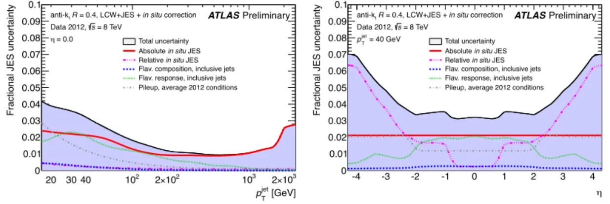
The residual of Jet Energy Scale calibration evaluated by the combination of these in-situ techniques is shown in Fig. 17, together with statistical and systematic uncertainties. All the measurements show consistent results and the maximum discrepancy is 3% in pT>1 TeV. The total uncertainty is 3% at the maximum. Including additional uncertainties due to pile-up and flavor response, a fractional uncertainty <2.5% is obtained for central jets with pT > 100 GeV as shown in Fig. 18 (left). The plot on the right shows the η dependence of JES uncertainty for jet with pT=40 GeV.

3.2.5 Pileup suppression

Low pT particles from multiple soft collisions (pile-up) increase the calorimeter activity and shift jet energies. To remove the energy shift, a pile-up correction has been developed based on the idea that noise (pile-up) has a lower energy density than signal jets [22]. “Median pT density” ρ, is defined as

(32)

[GeV] jet T p 20 30 40 102 2×102 103 MC / Response Data Response 0.9 0.92 0.94 0.96 0.98 1 1.02 1.04 1.06 1.08 1.1 _R_{= 0.4, LCW+JES} t anti-k Data 2012 ATLAS Preliminary | < 0.8 η = 8 TeV, | s +jet γ +jet Z Multijet

Total in situ uncertainty Statistical component

Figure 17: Residual of JES calibration obtained from the combination of the in-situ techniques with statistical and systematic uncertainties. This plot is cited from Ref. [21].

[GeV] jet T p 20 30 40 ₁₀2 ₁₀2 × 2 ₁₀3 ₁₀3 × 2

Fractional JES uncertainty

0 0.01 0.02 0.03 0.04 0.05 0.06 0.07 0.08 0.09 0.1 ATLAS Preliminary = 8 TeV s Data 2012, correction in situ = 0.4, LCW+JES + R t anti-k = 0.0 η Total uncertainty JES in situ Absolute JES in situ Relative

Flav. composition, inclusive jets Flav. response, inclusive jets Pileup, average 2012 conditions

η

-4 -3 -2 -1 0 1 2 3 4

Fractional JES uncertainty

0 0.01 0.02 0.03 0.04 0.05 0.06 0.07 0.08 0.09 0.1 ATLAS Preliminary = 8 TeV s Data 2012, correction in situ = 0.4, LCW+JES + R t anti-k = 40 GeV jet T p Total uncertainty JES in situ Absolute JES in situ Relative

Flav. composition, inclusive jets Flav. response, inclusive jets Pileup, average 2012 conditions

Figure 18: JES and additional uncertainties due to pile-up, flavor response and composition for central jets (left) and for jets with pT=40 GeV (right). These plots are cited from Ref. [21].

the median of pjet_T/Ajet _{of all the jets. Here, A}jet _{is the geometrical area of a jet which is determined jet} by jet by adding up all the clusters involved. The number of pile-up jets is much larger than jets from a hard collision, therefore the median is mainly determined by pile-up jets without a significant bias. Figure 19 (left) illustrates that ρ increases with the number of primary vertex per bunch crossing NPV. ρ provides a direct estimate of the global pile-up activity in any given event, while Ajet_{provides an estimate} of a jet’s sensitivity to pileup. By multiplying these two quantities, an estimate of the effects of pile-up is obtained. Subtracting this estimate from the original jet pTpermits to reduce the dependence on pile-up:

pjet,corr_T = pjet_T − ρ × Ajet. (46)

Figure 19 (right) shows the root-mean-square of (pjet,corr_T − ptrueT ) as a function of the average number of pileup interactions per bunch crossing 'µ(. The impact of pile-up on jet pTis evident from the linear rise observed in the uncorrected points. Compared to the previous offset correction method [23] based on 'µ( and NPVused in 2011, the jet area method further mitigates the degradation in jet pTresolution.

(33)

[GeV] ρ 0 5 10 15 20 25 30 Normalised entries 0 0.02 0.04 0.06 0.08 0.1 0.12 0.14 = 6 PV N NPV = 10 = 14 PV N NPV = 18 ATLAS Simulation < 21 〉 µ 〈 ≤ 20 = 8 TeV s Pythia Dijet 2012, LCW TopoClusters 〉 µ 〈 5 10 15 20 25 30 35 40 ) [GeV] true T - p reco T RMS(p 5 6 7 8 9 10 11 12 13 14 ATLAS Simulation =8 TeV s Pythia Dijet LCW R=0.6 t anti-k < 30 GeV true T p ≤ 20 | < 2.4 η | uncorrected ) correction PV , N 〉 µ 〈 f( A correction × ρ

Figure 19: (Left) ρ distribution for four representative values of the reconstructed Primary Vertex mul-tiplicity NPV. (Right) Root-mean-square width of the distributions of (preco_T − ptrue_T ) for anti-kT(R=0.6) jets. These plots are cited from Ref. [22].

3.2.6 b-tagging

Several tagging algorithms have been invented for better b-tagging efficiency. A method based on neural-network, MV1, which combines the inputs from IP3D, SV1 and JetFitter, is used to improve purity and efficiency.

IP3D[24] is the tagging algorithm using the likelihood technique in which input variables are com-pared with pre-defined distributions for both b- and light-jet hypotheses, obtained from Monte Carlo simulation. The signed transverse impact parameter significance and the longitudinal impact parameter significance, along with their correlation, are used as the input parameters.

SV1_{[24] is also an algorithm based on the likelihood technique, but using reconstructed Secondary} Vertex information. It uses ∆R between a jet and a b-hadron, and the number of two-track vertices. Also, the combined two-dimensional information of the Secondary Vertex mass and the energy fraction of the Secondary Vertex with respect to the total tracks are employed.

These methods have a drawback of giving a bad tagging efficiency in case a long-lived hadron is emitted from the decay as these methods assume only one Secondary Vertex. JetFitter [25] takes the decay of long-lived hadrons into consideration under the assumption that the long-lived hadron decays occur on the flight axis of the initial b-hadron. The separation between b-, c- and light-jets is performed based on the likelihood method.

MV1 algorithm combines the results from these methods using a neural-network. As the tagging efficiency is not critical in our analysis, we use a moderate working point at which 60% of b-jets are tagged. At this working point, light-jet rejection factor of 577, c-jet rejection factor of 8 and tau-jet rejection factor of 23 are obtained, respectively3_{. The discrepancy of the tagging efficiency between data} and Monte Carlo is corrected by applying a scale factor.

(34)

3.2.7 Object definition

Jet candidates defined in the previous section may contain “fake” jets. Here we apply further cleanings to define sets of genuine jets that are used in the analysis. Fake jets, such as cosmic muons, noise in the detector electronics and the particles not originating from the proton collision, are eliminated as follow.

• Pulse shapes of calorimeters are monitored for all jets. If the shape differs from the usual one, the jet may be a noise and is judged as a fake jet.

• The baseline voltage of LAr electronics takes some time to settle to the usual level after incoming of a jet. Instability of baseline voltage makes negative energy cells and if the total negative energy is sizable, the jet is tagged as a fake jet.

• The energy fraction of a radial layer in the total jet energy should be smaller than a specific thresh-old. If one layer has a significant fraction of the energy, it may be a fake jet produced by a scrapping particle, flying into the detector parallel to the beam axis.

Next, electron showers, which are also reconstructed as jets, are removed. Jet within ∆R < 0.2 from preselected electrons (defined in Table 4 for Hard electron and Table 5 for Soft electron) are removed.

Finally, we define four types of jets: signal jets, b-jets, Emiss

T jets and overlap removal jets. Signal jets are the ones on which our kinematic selections are applied. b-tagging is checked for signal jets with 60% efficiency working point to define b-jets. Emiss

T jets are the collection of jets with |η| < 2.5 and pT>20 GeV, which are defined to calculate E_Tmiss4. Overlap removal jets are defined to be used in the lepton isolation check, which will be discussed in Section 3.3.4. Table 2 summarizes their definitions.

Cut Value/description

Jet Type overlap removal Emiss

T signal b-jet

Acceptance pT>20 GeV pT >30 GeV

No limit on |η| |η| < 2.5

Overlap ∆R(jet, e) > 0.2

Other – MV1with 60% efficiency working point

Table 2: Summary of the jet selection criteria.

3.3 Electron

Electron reconstruction [26] starts from clustering electromagnetic calorimeter cells and then the cluster is matched to an inner detector track. As jets contain many tracks and calorimeter activities, raw electron candidates contain many “fake” electrons from jets, which are rejected by requiring additional quality selections such as Bremsstrahlung radiations in TRT and the absence of hadronic activity. Then we define several sets of electrons which are used in the following analysis.

3.3.1 Cluster reconstruction

Electron reconstruction begins with forming a seed cluster. A method called sliding window algo-rithm [17] with a window size of 3 × 5 in η × φ middle layer cell units (0.025 × 0.025), finds a seed cluster with energy above 2.5 GeV.

4_{Note that clusters between 2.5 < |η| < 4.9 are included in E}miss

T calculation as Soft term, which will be mentioned in