Baryonic flux in quenched and two-flavor dynamical QCD after Abelian projection

Baryonic flux in quenched and two‑flavor dynamical QCD after Abelian projection

著者 Bornyakov V.G., Ichie H., Mori Yoshihiro, Pleiter D., Polikarpov M.I., Schierholz G., Streuer T., Stuben H., Suzuki Tsuneo

journal or

publication title

Physical Review D

volume 70

number 5

page range 054506

year 2004‑01‑01

URL http://hdl.handle.net/2297/3482

Baryonic flux in quenched and two-flavor dynamical QCD after Abelian projection

V. G. Bornyakov,^1,2,3H. Ichie,^3,4Y. Mori,³D. Pleiter,⁵M. I. Polikarpov,²G. Schierholz,^5,6T. Streuer,^5,7H. Stu¨ben,⁸ T. Suzuki,³and DIK collaboration

1Institute for High Energy Physics, RU-142281 Protvino, Russia

2ITEP, B.Cheremushkinskaya 25, RU-117259 Moscow, Russia

3Institute for Theoretical Physics, Kanazawa University, Kanazawa 920-1192, Japan

4Tokyo Institute of Technology, Ohokayama 2-12-1, Tokyo 152-8551, Japan

5NIC/DESY Zeuthen, Platanenallee 6, D-15738 Zeuthen, Germany

6Deutsches Elektronen-Synchrotron DESY D-22603 Hamburg, Germany

7Institut fu¨r Theoretische Physik, Freie Universita¨t Berlin, D-14196 Berlin, Germany

8Konrad-Zuse-Zentrum fu¨r Informationstechnik Berlin, D-14195 Berlin, Germany

(Received 17 March 2004; revised manuscript received 15 June 2004; published 16 September 2004) We study the distribution of color electric flux of the three-quark system in quenched and full QCD (with Nf 2 flavors of dynamical quarks) at zero and finite temperature. To reduce ultraviolet fluctuations, the calculations are done in the Abelian projected theory fixed to the maximally Abelian gauge. In the confined phase we find clear evidence for aY-shape flux tube surrounded and formed by the solenoidal monopole current, in accordance with the dual superconductor picture of confinement. In the deconfined, high temperature phase monopoles cease to condense, and the distribution of the color electric field becomes Coulomb-like.

DOI: 10.1103/PhysRevD.70.054506 PACS numbers: 11.15.Ha, 12.38.Aw, 12.38.Gc

I. INTRODUCTION

So far most investigations of the static potential, and the dynamics that drives it, have concentrated on the quark-antiquark (QQ) system, while little is known about the forces of the three-quark (3Q) ensemble. For under- standing the structure of baryons and, in particular, for modeling the nucleon [1], it is important to learn about the forces and the distribution of color electric flux in the 3Qsystem as well. A particularly interesting question is whether a genuine three-body force exists and the con- fining flux tube is ofY-shape, or whether the long-range potential is simply the sum of two-body potentials, in agreement with a -Ansatz, resulting in a flux tube of -shape. By a flux tube ofY- and-shape we understand a flux tube between the three quarks having shortest possible length and a junction, and a flux tube constructed out of three-quark-antiquark flux tubes taken with a factor¹₂.

Several lattice quenched QCD studies report evidence for a-type long-range potential [2,3], while others claim a genuine three-body force [4,5]. In Ref. [4] various patterns of the three-quark system were considered with the distance between quarks in an equilateral triangle,d, up to 0.8 fm. It was found that at large distances the Y-Ansatz gives a better description of the three-quark potential than the-Ansatz. On the other hand, the au- thors of Ref. [5] found that at distances d <0:7 fm the three-quark potential is described quite well by-Ansatz, while it rises like the Y-Ansatz at larger distances, 0:7< d <1:5 fm.

The Y-Ansatz is also being supported by the field correlator method [6]. The difference between a - and

Y-shape potential is rather small and difficult to detect, because the underlying Wilson loop decays approximately exponentially with increasing interquark distance. A computation of the distribution of the color electric flux inside the baryon might help to resolve this problem.

In this paper we shall study the static potential and the flux tube of the 3Q system. The long-distance physics appears to be predominantly Abelian —being the result of a yet unresolved mechanism — and driven by mono- pole condensation. The use of Abelian variables is an essential ingredient in our work, as it leads to a substan- tial reduction of the statistical noise. Preliminary results of this investigation have been reported in Ref. [7].

The paper is organized as follows. In Sec. II we de- scribe the details of our simulation, including the corre- lation functions that we are going to compute. The results of the calculation are presented in Secs. III and IV.

Section III is devoted to the study of the 3Q system at zero temperature, while Sec. IV deals with the finite temperature case. Finally, in Sec. V we conclude.

II. SIMULATION DETAILS

We employ the Wilson gauge field action throughout this paper. In our studies of full QCD we are using non- perturbativelyOa improved Wilson fermions,

S_F S⁰_F i

2gc_SWa⁵X

s

s Fs s; (1) withN_f2flavors of dynamical quarks, whereS⁰_F is the ordinary Wilson fermion action. Further details of the dynamical runs are given in [8,9].

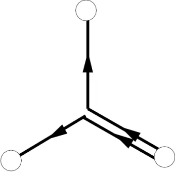
The system of three static quarks propagating fromA toBmay be described by the ‘‘baryonic’’ Wilson loop

W_3Q 1

3!"_ijk"_i⁰_j⁰_k⁰U_ii⁰C1U_jj⁰C2U_kk⁰C3; (2) where

UC Y

s;2C

Us; (3)

is the ordered product of link matricesU2SU3along the pathC, as shown in Fig. 1. The potential energy of this system is given by

V 1

L_T lim

L_T!1loghW_3Qi; (4) L_T being the temporal extent of the loop.

In the following we shall concentrate on Abelian var- iables, referring to the maximally Abelian gauge (MAG), and being obtained by standard Abelian projection [10,11]. To fix the MAG [12], we use a simulated anneal- ing algorithm described in [9]. We write the Abelian link variables as

us; diagu₁s; ; u₂s; ; u₃s; ;

u_is; expi"_is; (5) with

"_is; argU_iis; 1 3

X³

j1

argU_jjs; j_mod2#;

"_is; 2

4 3#;4

3#

:

(6)

They take values in U1 U1, and under a general gauge transformation they transform as

us; !ds^yus; ds;^ ds diagexpi$₁s;expi$₂s;

expi$₁s $₂s:

(7)

The Abelian Wilson loop is given by W_3Q^ab 1

3!j"_ijkju_iC1u_jC2u_kC3; (8) where uC is the Abelian counterpart of (3). W_3Q^ab is invariant under gauge transformations (7).

The physical properties of the 3Q system can be in- ferred from correlation functions of appropriate operators with the corresponding Wilson loop. Abelian operators take the form

Os diagO1s;O2s;O3s 2U1 U1: (9) For C-parity even operatorsO, like the action and mono- pole densities, the correlator of Os with the Abelian Wilson loop is given by [7,13]

hOsi3QhOsW_3Q^abi

hW^ab_3Qi hOi: (10) For C-parity odd operators, like the electric field and monopole current which carry a color index, the corre- lator is defined by

hOsi_3Q 1 3!

hOisj"_ijkju_iC1u_jC2u_kC3i

hW_3Q^abi ; (11) where summation overi; j; k is assumed. It is natural to use Wilson loop to study the static potential at zero temperature since it gives directly a singlet potential.

The Polyakov loop correlator gives in general a color- averaged potential, i.e., a mixture of the singlet and octet potentials, see e.g. [14]. At nonzero temperature one can use only the Polyakov loop correlator to study the static potential and we use the product P_3Q of three Polyakov loops closed around the boundary as baryonic source instead ofW_3Q:

P^ab_3Q 1

3!j"_ijkj‘_i~s₁‘_j~s₂‘_k~s₃; (12) where

‘_i~s Y^LT

s41

u_i~s; s₄;4 (13) FIG. 1. Three-quark Wilson loop.

V. G. BORNYAKOV, ET AL. PHYSICAL REVIEW D70054506

054506-2

is the Abelian Polyakov loop, L_T being the temporal extent of the lattice here. The correlators of Os with P_3Qare defined analogously to (10) and (11).

The observables we shall study are the action density (^3Q_A , the color electric fieldE^3Qand the monopole current k^3Q. The action density is given by

(^3Q_A s * 3

X

i;>

hcos"_is; ; i_3Q; (14) where

"_is; ; argu_is; ; ;

u_is; ; u_is; u_is; u^ ^y_is; u^ ^y_is;

(15) is the plaquette angle. The color electric field and mono- pole current correlators are defined by

E^3Qs; i ihdiag"₁s;4; i; "₂s;4; i; "₃s;4; ii_3Q (16) and

k^3Qs; 2#ihdiagk₁s; ; k₂s; ; k₃s; i_3Q; (17) wherek_is; is the monopole current [9,13].

The calculations in full QCD at zero temperature are performed on the24³48lattice at*5:29,0:1355, which corresponds to a pion mass ofm_#=m₍0:7and a lattice spacing of a=r₀0:18 [9] (i.e. a0:09 fm as- suming r₀0:5 fm). The calculations in full QCD at finite temperatureT are done on the16³8lattice at* 5:2 for various hopping parameters ranging from 0:1330 to 0:1360, which covers the temperature range [15] 0:8&T=T_c&1:2. The critical temperature T_c corresponds to 0:13441. At this we find m_#=m₍0:77. For comparison, we also did quenched simulations at zero temperature on the 16³32 lattice at

*6:0. At this * the lattice spacing is a=r₀ 0:186, i.e., it is roughly the same as on our full QCD lattices. To reduce the statistical noise we smeared the spatial links of the Abelian Wilson loop using ten sweeps of APE smear- ing [16] with$2, where$is a coefficient multiplying the sum of staples.

III. STATIC POTENTIAL AND BARYONIC FLUX AT ZERO TEMPERATURE

The minimalY-type distance between the quarks, i.e., the sum of the distance from the quarks to the Fermat point is [4]

L_Y 1

2 X

i>j

r²_ij2 3 p

S ₁₌₂

; (18)

where ~r_i marks the position of thei^th quark, r_ij j~r_i

~r_jjandSis the area of the triangle spanned by the three quarks. The Y-Ansatz predicts that the confining part of the baryonic potential is^3Q_Y L_Y, with string tension^3Q_Y equal to theQQ string tension [17]:

^3Q_Y ^QQ: (19)

The full expression describing both large and small dis- tances is

V^3QL_Y V₀^3QX

i<j

$^3Q

r_ij ^3Q_Y L_Y; (20) where, similarly to theQQ static potential,V₀^3Q is a self energy term, the Coulomb term with effective coupling

$^3Q comprises one gluon exchange as well as a Lu¨scher term, recently derived for the baryonic string in [18], and the confining term has string tension^3Q_Y . The-Ansatz prediction [19] is that the confining part of the potential is proportional to the perimeter of the triangle formed by the quarks

LX

i<j

j~r_i ~r_jj: (21) with string tension

^3Q 1

2^QQ: (22) The short distance part is of the same form as in Eq. (20).

Thus the full expression for the-Ansatz potential is V^3QL V₀^3QX

i<j

$^3Q

r_ij ^3Q L: (23) For short distances perturbation theory arguments relate the self energy and the Coulomb term coefficient to those of theQQ static potential [5]:

V₀^3Q 3

2V₀^QQ; $^3Q 1

2$^QQ: (24) On the other hand fitting the numerical data including both long and short distances by (20) or by (23) one may find results which differ from (24), e.g., due to the Lu¨scher term contribution. In Ref. [4] a rough agreement between the fit parameters and (24) has been found for both Y-Ansatz and-Ansatz fits.

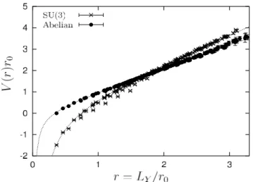
In Fig. 2 we show the baryon potential as a function of L_Y. An unphysical constantV₀^3Qhas been subtracted from the potentials. For equal distances between the quarks, i.e.

j~r_i~r_jj dL_Y= p3

for8ij, Eq. (20) becomes V^3QL_Y V₀^3Q3

3 p $^3Q

L_Y ^3Q_Y L_Y: (25) Fitting our data for three quarks in equilateral triangles by Eq. (25) for distances d <0:75 fm we found the Abelian string tension ^3Q_Y;aba²0:0381 and

0.0395(12) for the quenched and full theory, respectively.

These values agree within error bars with the Abelian string tension for theQQ flux tube^Q_ab^Q 0:0391and 0.0402(11) [9] thus supporting theY-Ansatz. Note, that both 3Q and QQ Abelian string tensions are slightly higher in full QCD. We found values for the self-energy and the Coulomb term coefficient smaller than prescribed by (24):V₀^3Q=V₀^QQ 1:285; $^3Q=$^QQ 0:274in full QCD and V₀^3Q=V₀^QQ 1:316; $^3Q=$^QQ 0:314 in quenched QCD. The fits are also shown in Fig. 2.

In Fig. 3 the Abelian and the nonAbelian quenched potentials are plotted together with respective fits. The data for the nonAbelian potential is taken from Ref. [4].

Comparison of ^3Q_Y;ab with the SU(3) result [4] gives ^3Q_Y;ab=^3Q_Y 0:833, which lends further support to the hypothesis of Abelian dominance.

If the confining flux is ofY-shape we would expect the long-distance part of the potential to be a universal func- tion of L_Y. In Fig. 4 we plot the Abelian potential as a function of L_Y (top), and as a function ofL (bottom).

The data show a universal behavior when plotted against L_Y. This is to a lesser extent the case when plotted against L, which supports a genuine three-body force of Y-type.

In Fig. 4 the fits by theY-Ansatz and by the-Ansatz for the quarks in the equilateral triangle are shown in the top and bottom parts, respectively. Note that for the quarks in the equilateral triangle these two fits are essentially the same with ^{3Q p1}₃^3Q_Y and equal self energy and Coulomb coefficient.

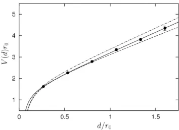
In Fig. 5 and 6 we show further comparison of our data with and Y-Ansa¨tze for full and quenched QCD. The data for the three-quark potential are plotted as a func-

FIG. 3. Comparison of the Abelian and SU(3) baryon poten- tial in the quenched approximation on the16³32lattice at* 6:0. The SU(3) potential is taken from [4].

FIG. 4. The Abelian baryon potential in full QCD, together with its monopole and photon part, as a function of L_Y (top) andL (bottom), respectively. The curves show fits (25) (top) and (23) (bottom) to the data with equal distances between the static sources.

FIG. 2. The Abelian baryon potential in full and quenched QCD.

V. G. BORNYAKOV, ET AL. PHYSICAL REVIEW D70054506

054506-4

tion of distance d for equilateral triangle. In the same figures the curves showing respective Y-Ansatz and -Ansatz predictions are plotted. We fix all parameters in the Ansa¨tze using relations (19), (22), and (24). We see that for both full and quenched QCD at distances d <

0:5 fm the three-quark potential data agree with the -Ansatz, while at larger distances it agrees with Y-Ansatz up to an additive constant indicating that the string tension^3Q_Y;ab is equal to^Q_ab^Q as was already dis- cussed above. Similar findings were presented for the quenched nonAbelian potential in [3]. Thus we conclude that our data for the Abelian potential confirm the Y-Ansatz for large distances. The agreement with the -Ansatz at short distances, which was also observed in [3], is probably a coincidence since the-Ansatz predic- tion Eq. (22) is formulated for large quark separations. On the other hand, the proximity of the potential to the -Ansatz at distances which are relevant for the spectrum calculations might be important for the phenomenolo- gists since the calculations with the -Ansatz potential are much simpler. The disagreement with theY-Anzatz at small distances was first clearly observed in Ref. [5]. One can guess that the finite size of the junction play the role in appearance of this discrepancy. Although our data for the static potential at small distances behave similar to that of Ref. [5] we are not in a position to make strong statements about the short distances since we are using the Abelian projection which, as many earlier observa- tions suggest, gives correct description of the static po- tentials at large distances only.

Although the results for the static potential are in favor of the Y-Ansatz, the difference from the-Ansatz pre-

diction is rather small. Thus it is worthwhile to study the color flux distribution. In Fig. 7 we show the distribution of the color electric fieldE~^3Q, and its surrounding mono- pole currentsk^3Q, on the 24³48lattice in full QCD. The time direction of the Wilson loop has been taken in one of the spatial directions of the lattice. Points on the hyper- plane orthogonal to the time direction of the Wilson loop are marked by x; y; z. The static quarks are placed at x; y; z 20;10;8, (25, 18, 8) and (30, 10, 8), respec- tively, i.e., they lie in thex; yplane. The color index of the electric field operator [cf. Equation (16)] is identified with the color index of the quark in the bottom-right corner (in the center bottom figure). Note that the sum of the electric field over the three color indices vanishes at any point. As expected, the flux emanates from the quark in the bottom-right corner and at about the center

FIG. 6. Same as Fig. 5 for quenched QCD.

FIG. 5. The Abelian three-quark potential and and Y-Ansa¨tze in full QCD for quarks in equilateral triangles as function of quark separation dL_Y=

p3

L=3. The solid line is a fit to the data, the dotted line is the -Ansatz prediction Eq. (23) and the dashed line is the Y-Ansatz pre- diction Eq. (25). For both Ansa¨tze Eq. (24) was used.

FIG. 7. Distribution of the color electric fieldE~^3Qin thex; y plane on the24³48lattice (center bottom figure), together with the monopole currents k^3Qin the x; zand y; zplanes (ad- jacent figures), respectively, at the position marked by the respective solid lines. The magnitude of E^3Q and k^3Q is in- dicated by the length of the arrows.

of the3Qsystem splits into two parts. The flux lines are schematically drawn in Fig. 8. A similar picture holds for the top and bottom-left quark and their respective fluxes.

In the adjacent figures we show the monopole current in the planes perpendicular to the electric flux lines, i.e., the x; zandy; zplanes. They form a solenoidal current, as in the case of theQQ system, in agreement with the dual superconductor picture of confinement.

We may decompose the Abelian gauge field into a monopole and photon part according to the definition [20,21]

"_is; "^mon_i s; "^ph_i s; ;

"^mon_i s; 2#X

s⁰

Dss⁰r$ m_is⁰; $; ; (26)

where Ds ¹s is the lattice Coulomb propagator, r is the lattice backward derivative, and m_is; ; counts the number of Dirac strings piercing the plaquette u_is; ; . If one computesk_is; from"^mon_i s; one recovers almost all monopole currents. In Fig. 4 we see that the monopole part is largely responsible for the linear behavior of the potential, as was found already in case of the QQ potential [9]. The ratio of monopole to Abelian string tension turns out to be 0.81(3).

In Fig. 9 we show the distribution of the Abelian color electric field and its monopole and photon parts. The photon part shows a Coulomb-like distribution, while the monopole part has no sources. Outside the flux tube the monopole and photon parts of the color electric field

largely cancel. The middle figure shows clearly that the flux lines are attracted to aY-type geometry.

In Fig. 10 we show the action density (^3Q_A of the 3Q system in full QCD. Also shown is the monopole and photon part of(^3Q_A separately. Let us first look at the (full) Abelian density. It clearly displays aY-type geometry of the color forces. This is, of course, indistinguishable from a geometry of purely two-body forces with strongly at- tracting flux lines. The monopole part of the action den- sity shows no sources. Apart from that, it appears that the action density originates almost entirely from the mono- pole part. The sources show up in the photon part of the action density as expected.

FIG. 8. Schematic view of the color electric field.

FIG. 9. Distribution of the Abelian color electric field E~^3Q (top) broken into monopole (middle) and photon parts (bottom) on the24³48lattice in full QCD. The color index of the electric field operators corresponds to that of the quark in the bottom- right corner. Only part of the lattice is shown here.

V. G. BORNYAKOV, ET AL. PHYSICAL REVIEW D70054506

054506-6

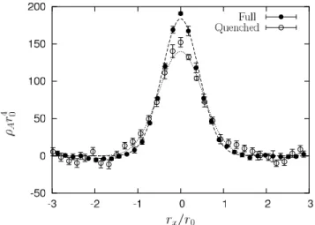
We have done similar calculations (to the ones shown in Figs. 4, 7, 9, and 10) in quenched QCD as well. Part of our findings have been reported in [7], and we refrain from repeating them here. Qualitatively, we found the same results as in full QCD at m_#=m₍0:7. In Fig. 11 we compare the action density of full and quenched QCD.

We see that at the center of the flux tube the action density

in full QCD is slightly higher than for the quenched case, while the shapes are rather similar. The same feature has been observed for theQQ flux tube [9]. We have estimated the width2of the flux tube using a Gaussian fit [9]. The result is 20:304fm and 0.36(11) fm in full and quenched QCD, respectively. This is to be compared with the width of theQQ flux tube, which turned out to be 0.29(1) fm in full and quenched QCD [9]. We found that the width increases closer to the junction. So the numbers quoted above are only to tell that the width of the baryon flux tube, away from the junction is not very different from that of theQQ flux tube. For a more precise deter- mination of the width larger quark separation is necessary.

It is interesting to compare the action density shown in Fig. 10 with the action density constructed out of three QQ flux tube action densities multiplied, in agreement with (22), by a factor ¹₂ to take into account that we are dealing with pairs of quarks rather than with QQ pairs.

Such a comparison has been done in Ref. [5] for the Potts model. For theQQ action density we used the results of Ref. [9]. The resulting density is shown in Fig. 12.

Figures 10 and 12 look rather different. The most impor- tant difference is that the measured density has a bump in the center, while the -Ansatz density has a dip. This comparison gives further support to theY-Ansatz.

IV. BARYONIC FLUX AT FINITE TEMPERATURE

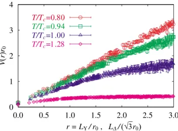
We expect the flux tube to disappear and the color electric field to become Coulomb- or Yukawa-like above the finite temperature phase transition T_c and when the string breaks in full QCD. This phenomenon has been observed in case of the QQ system in the pure SU(2) gauge theory for temperatures T > T_c [22] and in full QCD forTjust below and aboveT_c [23]. Throughout this Section we shall use the Polyakov loop (12) to create a baryon.

In Fig. 13 we show the baryon potential on the 16³8 lattice at*5:2for several values of. At this*value

T /exp2:81=: (27)

FIG. 11. The action density(^3Q_A r⁴₀of Fig. 10 plotted across the flux tube at the distance3afrom the quark and 2a from the junction.

30 40 50 60 70

20 25 30 35 40 45 50

FIG. 12. The Abelian action density of the 3Q system as predicted by the-Ansatz in full QCD.

17.5 20 22.5 25 27.5 30 32.5 6

8 10 12 14 16 18 20

17.5 20 22.5 25 27.5 30 32.5 6

8 10 12 14 16 18 20

17.5 20 22.5 25 27.5 30 32.5 6

8 10 12 14 16 18 20

FIG. 10. The Abelian action density of the3Qsystem in full QCD, together with the monopole and photon part.

Increasingthus increases the temperature. We cross the finite temperature phase transition at0:1344[15]. We see that the potential flattens off while we approach the transition point. However, the distances we were able to probe are not large enough to make any statement about string breaking.

To compute the action density(^3Q_A and the electric field and monopole correlators E^3Q and k^3Q, respectively, we need to reduce the statistical noise. We do that by averag- ing over time slices and using extended operators

(^3Q_A s!1

8f(^3Q_A s (^3Q_A s^1^2^3 (^3Q_A s^1^2 (^3Q_A s^1^3 (^3Q_A s^2^3 (^3Q_A s^1

(^3Q_A s^2 (^3Q_A s^3g; (28)

E^3Qs; i!1

2fE^3Qs; i E^3Qsi; ig;^ (29)

k^3Qs; !1

2fk^3Qs; k^3Qs^2; g; 1;3 (30) where (again) we have assumed that the quarks lie in the x; yplane, and we consider the monopole current in the z; xplane.

In Fig. 14 we plot the Abelian action density in the deconfined phase at 0:1360. As was to be expected, the action density shows three Coulomb-like peaks at the position of the quarks, similar to the photon part of the action density at zero temperature as shown in Fig. 10.

In Fig. 15 we show the monopole part of the electric field, averaged over the color components, and the ac- companying monopole current for three values of , corresponding (from left to right) to the confined case, toTT_cand to the deconfined phase. In the confinement phase (0:1335) we find the flux to be of Y-shape, similar to the zero temperature case where we used Wilson loop correlators. Note that the Polyakov lines do not have a Y-shape junction like the Wilson loop does, which excludes the possibility that the flux is being induced by the color lines. Just below T_c (0:1344) we still see aY-shape flux, while in the deconfined phase (0:1360) the electric field becomes Coulomb-like.

V. CONCLUSIONS

We have studied the 3Q system in the maximally Abelian gauge in full QCD at zero and at finite tempera- ture. Among the quantities we have looked at are the Abelian baryon potential as well as the flux distribution and the action density. While on the basis of the potential

2.5 5 7.5 10 12.5 15 2.5

5 7.5 10 12.5 15

FIG. 14 (color online). The Abelian action density in the deconfined phase at0:1360.

FIG. 15 (color online). The color electric field (top) and monopole currents (bottom) on the16³8lattice at0:1335 (left), 0.1344 (middle) and 0.1360 (right). The three quarks lie in (what we call) thex; yplane. The bottom figures show the monopole currents in thex; zplane at the position marked by the solid lines in the top figures.

0 1 2 3 4

0.0 0.5 1.0 1.5 2.0 2.5 3.0

V(r)r0

r = L_Y /r₀ , L_∆ /(√3r₀) T/T_c=0.80

T/Tc=0.94 T/T_c=1.00 T/Tc=1.28

FIG. 13 (color online). The monopole part of the baryon potential at finite temperature in full QCD as a function of L_Y(TT_c) andL (T > T_c), respectively.

V. G. BORNYAKOV, ET AL. PHYSICAL REVIEW D70054506

054506-8

it is hard to decide whether the long-range potential is of - orY-type, the distribution of the color electric field and the action density clearly shows aY-shape geometry.

As in theQQ system, we identified the solenoidal mono- pole current to be responsible for squeezing the color electric flux into a narrow tube. Little difference to the quenched theory was found. In the deconfined phase the flux tube disappears, and the color electric field assumes a Coulomb-like form. Our results are in qualitative agree- ment with the predictions of the dual Ginzburg-Landau model [24]: the baryon flux hasY-shape, and the sole- noidal monopole currents are clearly observed.

ACKNOWLEDGMENTS

The dynamical gauge field configurations at T0 have been generated on the Hitachi SR8000 at LRZ

Munich. We thank the operating staff for their support.

The dynamical gauge field configurations at T >0 have been generated on the Hitachi SR8000 at KEK Tsukuba.

The analysis has largely been done on the COMPAQ Alpha Server ES40 at Humboldt University, as well as on the NEC SX5 at RCNP Osaka. We wish to thank M. N.

Chernodub, M. Mu¨ller-Preussker, Y. Koma and H.

Suganuma for useful discussions. H. I. thanks the Humboldt University and Kanazawa University for hos pitality. V. B. is supported by JSPS. T. S. is supported by JSPS Grant-in-Aid for Scientific Research on Priority Areas 13135210 and 15340073. M. I. P. is supported by grant Nos. RFBR 02-02-17308, RFBR 01-02-17456, INTAS-00-00111, DFG-RFBR 436 RUS 113/739/0, RFBR-DFG 03-02-04016 and CRDF grant no. RPI- 2364-MO-02.

[1] S. Capstick and N. Isgur, Phys. Rev. D34, 2809 (1986).

[2] G. S. Bali, Phys. Rep.343, 1 (2001).

[3] C. Alexandrou, Ph. de Forcrand, and A. Tsapalis, Phys.

Rev. D65, 054503 (2002).

[4] T. T. Takahashi, H. Suganuma, Y. Nemoto, and H.

Matsufuru, Phys. Rev. D 65, 114509 (2002); T. T.

Takahashi, H. Matsufuru, Y. Nemoto, and H.

Suganuma, Phys. Rev. Lett.86, 18 (2001).

[5] C. Alexandrou, Ph. de Forcrand, and O. Jahn, Nucl. Phys.

(Proc. Suppl.)119, 667 (2003).

[6] D. S. Kuzmenko and Yu. A. Simonov, Phys. Lett. B494, 81(2000); Yad. Fiz. 67, 561 (2004) [Phys. At. Nucl.67, 543 (2004)].

[7] H. Ichie, V. Bornyakov, T. Streuer, and G. Schierholz, Nucl. Phys. (Proc. Suppl.)119, 751 (2003); Nucl. Phys. A 721, 899 (2003).

[8] H. Stu¨ben, Nucl. Phys. (Proc. Suppl.)94, 273 (2001).

[9] DIK Collaboration, V. G. Bornyakov, hep-lat/0310011.

[10] G. ’t Hooft, Nucl. Phys.B190, 455 (1981).

[11] A. S. Kronfeld, M. L. Laursen, G. Schierholz, and U.-J.

Wiese, Phys. Lett. B198, 516 (1987).

[12] F. Brandstaeter, G. Schierholz, and U.-J. Wiese, Phys.

Lett. B272, 319 (1991).

[13] V. Bornyakov, H. Ichie, S. Kitahara, Y. Koma, Y. Mori, Y.

Nakamura, M. Polikarpov, G. Schierholz, T. Streuer, H.

Stu¨ben, and T. Suzuki, Nucl. Phys. (Proc. Suppl.) 106, 634 (2002).

[14] S. Nadkarni, Phys. Rev. D33, 3738 (1986).

[15] DIK Collaboration, V. G. Bornyakov et al., hep-lat/

0401014.

[16] APE Collaboration M. Albaneseet al., Phys. Lett. B192, 163 (1987).

[17] J. Carlson, J. B. Kogut, and V. R. Pandharipande, Phys.

Rev. D27, 233 (1983).

[18] O. Jahn and P. de Forcrand, Nucl. Phys. (Proc. Suppl.) 129-130, 700 (2004).

[19] J. M. Cornwall, Phys. Rev. D54, 6527 (1996).

[20] J. Smit and A. van der Sijs, Nucl. Phys.B355, 603 (1991).

[21] T. Suzuki, S. Ilyar, Y. Matsubara, T. Okude, and K.Yotsuji, Phys. Lett. B 347, 375 (1995); 351, 603(E) (1995).

[22] Y. Peng and R.W. Haymaker, Phys. Rev. D 52, 3030 (1995).

[23] V. Bornyakov, H. Ichie, Y.Koma, Y. Mori, Y. Nakamura, M. Polikarpov, G. Schierholz, T. Streuer, and T. Suzuki, Nucl. Phys. (Proc. Suppl.)119, 712 (2003).

[24] M. N. Chernodub and D. A. Komarov, JETP Lett.68, 117 (1998); Y. Koma, E.-M. Ilgenfritz, T. Suzuki, and H. Toki, Phys. Rev. D64, 014015 (2001).